INTRODUCTION

A major advantage of analyzing circuits using Kirchhoff’s law as we did in Chapter 3 is that we can analyze a circuit without tampering with its original configuration. A major disadvantage of this approach is that, for a large, complex circuit, tedious computation is involved.

The growth in areas of application of electric circuits has led to an evolution from simple to complex circuits. To handle the complexity, engineers over the years have developed some theorems to simplify circuit analysis. Such theorems include Thevenin’s and Norton’s theorems. Since these theorems are applicable to linear circuits, we first discuss the concept of circuit linearity. In addition to circuit theorems, we discuss the concepts of superposition, source transformation, and maximum power transfer in this chapter. The concepts we develop are applied in the last section to source modeling and resistance measurement.

LINEARITY PROPERTY

Linearity is the property of an element describing a linear relationship between cause and effect. Although the property applies to many circuit elements, we shall limit its applicability to resistors in this chapter. The property is a combination of both the homogeneity (scaling) property and the additive property.

The homogeneity property requires that if the input (also called the excitation) is multiplied by a constant, then the output (also called response) is multiplied by the same constant. For a resistor, for example, Ohm’s law relates the input I to the output v,

If the current is increased by constant k, then the voltage increases correspondingly by k, that is,

The additive property requires that the response to a sum of inputs is the sum of the responses to each input applied separately. Using the voltage current relationship of a resistor, if

and

then applying $(i_1+i_2)$ gives

We say that a resistor is a linear element because the voltage-current relationship satisfies both the homogeneity and the additive properties.

In general, a circuit is linear if it is both additive and homogeneous. A linear circuit consists of only linear elements, linear dependent sources, and independent sources.

A linear circuit is one whose output is linearly related (or directly proportional) to its input.

Note that since $p=i^{2}R=v^2/R$ (making it a quadratic function rather than a linear one), the relationship between power and voltage (or current) is nonlinear. Therefore, the theorems covered in this chapter are not applicable to power.

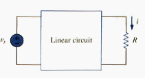
To illustrate the linearity principle, consider the linear circuit shown in [link]. The linear circuit has no independent sources inside it. It is excited by a voltage source vs, which serves as the input. The circuit is terminated by a load R. We may take the current i through R as the output. Suppose $v_S=\text{10}V$ gives i = 2 A. According to the linearity principle, $v_S=\mathrm{1V}$ will give i = 0.2 A. By the same token, i = 1 mA must be due to $v_S=5\text{mV}$.

SUPERPOSITION

If a circuit has two or more independent sources, one way to determine the value of a specific variable (voltage or current) is to use nodal or mesh analysis as in Chapter 3. Another way is to determine the contribution of each independent source to the variable and then add them up. The latter approach is known as the superposition.

The idea of superposition rests on the linearity property.

The superposition principle states that the voltage across (or current through) an element in a linear circuit is the algebraic sum of the voltages across (or currents through) that elements due to each independent source acting alone.

The principle of superposition helps us to analyze a linear circuit with more than one independent source by calculating the contribution of each independent source separately. However, to apply the superposition principle, we must keep two things in mind.

1. We consider one independent source at a time while all other independent sources are turned off. This implies that we replace every voltage source by 0 V (or a short circuit), and every current source by 0 A (or an open circuit). This way we obtain a simpler and more manageable circuit.

2. Dependent sources are left intact because they are controlled by circuit variables.

With this in mind, we apply the superposition principle in three steps:

Steps to apply superposition principle:

1. Turn off all independent sources except one source. Find the output (voltage or current) due to that active source using the techniques covered in Chapters 2 and 3.
2. Repeat step 1 for each of the other independent sources.

Find the total contribution by adding algebraically all the contributions due to the independent sources.

Analyzing a circuit using superposition has one major disadvantage: it may very likely involve more work. If the circuit has three independent sources, we may have to analyze three simpler circuits each providing the contribution due to the respectively individual source. However, superposition does help reduce a complex circuit to simpler circuits through replacement of voltage sources by short circuits and of current sources by open circuits.

Keep in mind that superposition is based on linearity. For this reason, it not applicable to the effect on power due to each source, because the power absorbed by a resistor depends on the square of the voltage or current. If the power value is needed, the current through (or voltage across) the element must be calculated first using superposition.

SOURCE TRANSFORMATION

We have noticed that series-parallel combination and wye-delta transformation help simplify circuits. Source transformation is another tool for simplifying circuits. Basic to these tools is concept of equivalence. We recall that an equivalent circuit is one whose v-i characteristics are identical with the original circuit.

In Section 3.6, we saw that node-voltage (or mesh current) equations can be obtained by mere inspection of a circuit when the sources are all independent current (or all independent voltage) sources. It is therefore expedient in circuit analysis to be able to substitute a voltage source in series with a resistor for a current source in parallel with a resistor, or vice versa, as shown in [link]. Either substitution is known as source transformation.

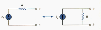
A source transformation is the process of replacing a voltage source vs in series with a resistor R by a current source is in parallel with a resistor R, or vice versa.

The two circuits in [link] are equivalent – provided they have the same voltage–current relation at terminals a-b. It is easy to show that they are indeed equivalent. If the sources are turned off, the equivalent resistance at terminals a-b in both circuits is R. Also, when terminals a-b are short circuited, the short circuit current flowing from a to b is $i_{\text{SG}}=v_S/R$ in the circuit in the left hand side and $i_{\text{SG}}=i_S$ for the circuit on right hand side. Thus, $v_S/R=i_S$ in order for the two circuits to be equivalent. Hence, source transformation requires that

or

$i_S=\frac{v_S}{R}$

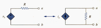
Source transformation also applies to dependent sources, provided we carefully handle the dependent variable. As shown in [link], a dependent voltage source in series with a resistor can be transformed to a dependent current source in parallel with the resistor or vice versa where we make sure that [link] is satisfied.

Like wye-delta transformation we studied in Chapter 2, a source transformation does not affect the remaining part of the circuit. When applicable, source transformation is a powerful tool that allows circuit manipulations to ease circuit analysis. However, we should keep the following points in mind when dealing with source transformation.

1. Note from [link] (or [link]) that the arrow of the current source is directed toward the positive terminal of the voltage source.

2. Note from [link] that source transformation is not possible when R = 0, which is the case with an ideal voltage source. However, for a practical, nonideal voltage source, . Similarly, an ideal current source with $R=\infty$ cannot be replaced by a finite voltage source.

THEVENIN’S THEOREM

It often occurs in practice that a particular element in the circuit is variable (usually called the load) while other elements are fixed. As a typical example, a household outer terminal may be connected to different appliances constituting a variable load. Each time the variable element is changed, the entire circuit has to be analyzed all over again. To avoid this problem, Thevenin’s theorem provides a technique by which the fixed part of the circuit is replaced by an equivalent circuit.

According to Thevenin’s theorem, the linear circuit in [link](a) can be replaced by that in [link](b). The load in [link] may be a single resistor or another circuit. The circuit to the left of the terminals a-b in [link](b) is known as the Thevenin equivalent circuit; it was developed in 1883 by M. Leon Thevenin (1857-1926), a French telegraph engineer.

Thevenin’s theorem states that a linear two-terminal circuit can be replaced by an equivalent circuit consisting of a voltage source $V_{\text{Th}}$ in series with a resistor $R_{\text{Th}}$, where $V_{\text{Th}}$ is the open-circuit voltage at the terminals and $R_{\text{Th}}$ is the input or equivalent resistance at the terminals when the independent sources are turned off.

The proof of the theorem will be given later, in section 7. Our major concern right now is how to find the Thevenin equivalent voltage $V_{\text{Th}}$ and resistance $R_{\text{Th}}$. To do so, suppose the two circuits in [link] are equivalent. Two circuits are said to be equivalent if they have the same voltage-current relation at their terminals. Let us find out what will make open-circuits in [link] equivalent. If the terminals a-b are made open-circuit voltage (by removing the load), no current flows, so that the open-circuit voltage across the terminals a-b in [link](a) must be equal to the voltage source $V_{\text{Th}}$ in [link](b), since the two circuits are equivalent. Thus $V_{\text{Th}}$ is open-circuit voltage across the terminals as shown in [link](a); that is,

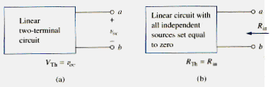
Again, with the load disconnected and terminals a-b open-circuited, we turn off all independent sources. The input resistance (or equivalent resistance) of the dead circuit at the terminals a-b in [link](a) must be equal to $R_{\text{Th}}$ in [link](b) because the two circuits are equivalent. Thus, $R_{\text{Th}}$ is the input resistance at the terminals when the independent sources are turned off, as shown in [link](b), that is,

To apply this idea in finding the Thevenin resistance $R_{\text{Th}}$, we need to consider two cases,

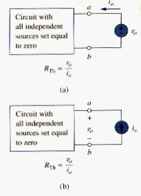
CASE 1. If network has no dependent sources, we turn off all independent sources, $R_{\text{Th}}$ is the input resistance of the network looking between terminals a and b, as shown in [link](b).

CASE 2. If the network has dependent sources, we turn off all independent sources. As with superposition, dependent sources are not to be turned off because they are controlled by circuit variables. We apply a voltage sources v0 at terminals a and b and determine the resulting current i0. Then $R_{\text{Th}}=v_0/i_0$, as shown in [link](a). Alternatively, we may insert a current source i0 and at terminals a-b as shown in [link](b) and find the terminal voltage $v_0$. Again $R_{\text{Th}}=v_0/i_0$. Either of the two approaches will give the same result. In either approach we may assume any value or $v_0$ and $i_0$. For example, we may use $v_0=\mathrm{1V}$ or $i_0=\mathrm{1A}$, or even use unspecified values of $v_0$ or $i_0$.

It often occurs that $R_{\text{Th}}$ takes a negative value. In this case, the negative resistance (v = - iR) implies that the current is supplying power. This is possible in a circuit with dependent sources.

Thevenin’s theorem is very important in circuit analysis. It helps simplify a circuit. A large circuit may be replaced by a simple independent voltage source and a single resistor. This replacement technique is powerful tool in circuit design.

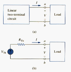
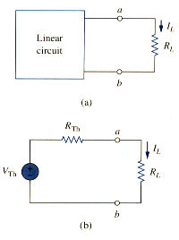
As mentioned earlier, a linear circuit with a variable load can be replaced by the Thevenin equivalent, exclusive of the load. The equivalent network behaves the same way externally as the original circuit. Consider a linear circuit terminated by a load $R_L$, as shown in [link](a). The current $I_L$through the load and the voltage $V_L$across the load are easily determined once the Thevenin equivalent of the current at the load’s terminals is obtained, as shown in [link](b). From [link](b), we obtain

Note from [link](b) that the Thevenin equivalent is a simple voltage divider, yielding $V_L$ by mere inspection.

NORTON’S THEOREM

In 1926 about 43 years after Thevenin published his theorem. E. L. Norton, an American engineer at Bell Telephone Laboratories, proposed a similar theorem.

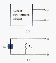
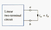
Norton theorem states that a linear two-terminal circuit can be replaced by an equivalent circuit consisting of a current source $I_N$ in parallel with a resistor $R_N$, where $I_N$ is the short-circuit current through the terminals and $R_N$ is the input or equivalent resistance at the terminals when the independent sources are turned off.

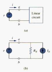
Thus, the circuit in [link](a) can be replaced by the one in [link](b).

The proof of Noton’s theorem will be given in the next section. For now, we are mainly concerned with how to get $R_{\text{N}}$ and $I_{\text{N}}$. We find $R_{\text{N}}$. in the same way we find $R_{\text{Th}}$. In fact, from what we know about source tranformation, the Thevenin and Norton resistances are equal; that is,

To find the Norton current IN, we determine the short-circuit current flowing from terminal a to b in both circuits in [link]. It is evident that the circuit the short-circuit current in [link](b) is IN. this must be the same short-circuit current from terminal a and b in [link](a), since the two circuits are equivalent. Thus,

shown in [link]. Dependent and independent sources are treated the same way as in Thevenin’s theorem.

Observe the close relationship between Norton’s and Thevenin’s theorems: $R_N=R_{\text{Th}}$ as in [link], and

This is essentially source transformation. For this reason, source transformation is often called Thevenin-Norton transformation.

Since $V_{\text{Th}}$, $I_N$ and $R_{\text{Th}}$ are related according to [link], to determine the Thevenin or Norton equivalent circuit requires that we find:

• The open-circuit voltage $v_{\text{oc}}$ across terminal a and b.
• The short-circuit current $i_{\text{SG}}$ at terminals a and b.
• The equivalent or input resistance $R_{\text{in}}$ at terminals a and b when all independent sources are turned off.
• We can calculate any two of the three using the method that takes the least effort and use them to get the third using Ohm’s law. Also, since

$R_{\text{Th}}=\frac{v_{\text{oc}}}{i_{\text{sc}}}=R_N$

the open-circuit and short circuit tests are sufficient to find any Thevenin or Norton equivalent.

DERIVATIONS OF THEVENIN’S AND NORTON’S THEOREMS

In this section, we will prove Thevenin’s and Norton’s theorem using the superposition principle.

Consider the linear circuit in [link](a). It is assumed that the circuit contains resistors, and dependent and independent sources. We have access to the circuit via terminals a and b, through which current from an external source is applied. Our objective is to ensure that the voltage-current relation at terminals a and b is identical to that of the Thevenin equivalent in [link](b). For the sake of simplicity, suppose the linear circuit in [link](a) contains two independent voltage sources vs1 and vs2 and two independent current sources $i_{\mathrm{S1}}$ and $i_{\mathrm{S1}}$. We may obtain any circuit variable, such as the terminal voltage v, by applying superposition. That is, we consider the contribution due to each independent source including the external source i. by superposition, the terminal voltage v is

Where $A_0$, $A_1$, $A_2$, $A_3$, and $A_4$ are constants. Each term on the right hand side of [link] is the contribution of the related independent source; that is, $A_{0}i$ is contribution to v due to the voltage source $v_{\mathrm{S1}}$, and so on. We may collect terms for the internal independent sources together as $B_0$, so that [link] become

Where $B_0=A_1{v}_{\mathrm{s1}}+A_2{v}_{\mathrm{s2}}+A_3{i}_{\mathrm{s1}}+A_4{i}_{\mathrm{s2}}$. We now want to evaluate the values of constants $A_0$ and $B_0$. When the terminals a and b are open-circuited, i = 0 and $v=B_0$. thus B0 is open-circuit voltage $v_{\text{oc}}$, which is the same as $V_{\text{Th}}$, so

When all the internal sources are turned off, $B_0=0$. The circuit can then be replaced by an equivalent resistance $R_{\text{eq}}$, which is the same as $R_{\text{Th}}$, and [link] becomes

Substituting the values of $A_0$ and $B_0$ in [link] gives

which expresses the voltage-current relation at terminals a and b of the circuit in [link](b). Thus, the two circuits in [link](a) and [link](b) are equivalent.

When the same linear circuit is driven by a voltage source v as shown in [link](a), the current flowing into the circuit can be obtained by superposition as

Where $C_{0}v$ is the contribution to i due to the external source v and $D_0$ contains the contributions to i due to all independent sources. When the terminals a-b are short-circuited, v = 0 so that $i=D_0=-i_{\text{SG}}$, where $i_{\text{SG}}$ is the short-circuit current flowing out of terminal a, which is the same Norton current $I_N$, i.e.,

When all terminal independent sources are turned off, $D_0=0$ and the circuit can be replaced by an equivalent resistance $R_{\text{eq}}$ (or an equivalent conductance $G_{\text{eq}}=1/R_{\text{eq}}$), which is the same as $R_{\text{Th}}$ or $R_N$. Thus [link] becomes

This expresses the voltage-current relation at terminals a-b of the circuit in [link](b), confirming that the two circuits in [link](a) and [link](b) are equivalent.

MAXIMUM POWER TRANSFER

In many practical situations, a circuit is designed to provide power to a load. There are applications in areas such as communications where it is desirable to maximize the power delivering the maximum power to a load when given a system with known internal losses. It should be noted that this will result in significant internal losses greater than or equal to the power delivered to the load.

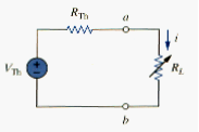
The Thevenin equivalent is useful in finding the maximum power a linear circuit can deliver to a load. We assume that we can adjust the load resistance $R_L$. If the entire circuit is replaced by its Thevenin equivalent except for the load, as shown in [link], the power delivered to the load is

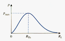
For a given circuit, $V_{\text{Th}}$ and $R_{\text{Th}}$ are fixed. By varying the load resistance $R_L$, the power delivered to the load varies as sketched in [link]. We notice from [link] that the power is small for small or large values of RL but maximum for some value of $R_L$ between 0 and $\infty$. We now want to show that this maximum power occurs when $R_L$ is equal to $R_{\text{Th}}$. This is known as the maximum power theorem.

Maximum power is transferred to the load when the load resistance equals the Thevenin resistance as seen from the load ( $R_L=R_{\text{Th}}$).

To prove the maximum power transfer theorem, we differentiate p in [link] with respect to $R_L$ and set the result equal to zero. We obtain

$\frac{\text{dp}}{{\text{dR}}_L}=V_{\text{Th}}^2[\frac{(R_{\text{Th}}+R_L{)}^2-{\mathrm{2R}}_L(R_{\text{Th}}+R_L)}{(R_{\text{Th}}+R_L{)}^4}]=V_{\text{Th}}^2[\frac{(R_{\text{Th}}+R_L-{\mathrm{2R}}_L)}{(R_{\text{Th}}+R_L{)}^3}=0$

This implies that

Which yields

Showing that the maximum power transfer takes place when the load resistance $R_L$ equal the Thevenin resistance RTh. We can readily confirm that [link] gives the maximum power by showing that

The maximum power transferred is obtained by substituting [link] into [link], for

[link] applies only when $R_L=R_{\text{Th}}$. When , we compute the power delivered to the load using [link].

APPLICATIONS

I this section we will discuss two important practical applications of the concepts covered in this chapter: source modeling and resistance measurement.

Source modeling

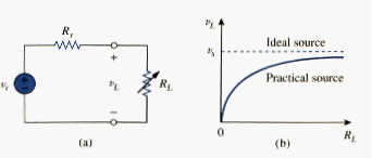
Source modeling provides an example of the usefulness of the Thevenin or the Norton equivalent. An active source such as a battery is often characterized by its Thevenin or Norton equivalent circuit. An ideal voltage source provides a constant voltage irrespective of the current drawn by the load, while an ideal current source supplies a constant current regardless of the load voltage. As [link] shows practical voltage and current sources are not ideal, due to their internal resistances or source resistances $R_s$ and $R_p$. They become ideal as $R_S\to 0$ and $R_p\to \infty$. To show that this is the case, consider the effect of the load on voltage sources, as shown in [link](a). By the voltage division principle, the load voltage is

$v_L=\frac{R_L}{R_s+R_L}{v}_s$

As $R_L$ increase, the load voltage approaches a source voltage $v_S$, as illustrated in [link](b). from [link], we should note that:

1. The load voltage will be constant if the internal resistance $R_S$ of the source is zero or, at least, . In other words, the smaller $R_S$ is compared to $R_L$, the closer the voltage source is to being ideal.
2. When the load is disconnected (i.e., the source is open-circuit so that $R_L\to \infty$), $v_{\text{oc}}=v_s$. Thus $v_s$ may be regarded as the unloaded source voltage. The connection of the load causes the terminal voltage to drop in magnitude; this is known as the loading effect.

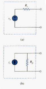
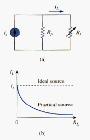
The same argument can be made for a practical current source when connected to a load as shown in [link]. By the current division principle,

$i_L=\frac{R_p}{R_p+R_L}{i}_s$

[link] shows the variation in the load current as the load resistance increases. Again, we notice a drop in current due to the load (loading effect), and load current is constant (ideal current source) when the internal resistance is very large (i.e., $R_F\to \infty$ or, at least, $R_p\text{>>}{R}_L$).

Sometimes, we need to know the unloaded source voltage $v_s$ and the internal resistance $R_s$ of a voltage source. To find $v_s$ and $R_s$, we follow the procedure illustrated in [link]. First, we measure the open-circuit voltage $v_{\text{oc}}$ as in [link](a) and set

$V_S=V_{\text{oc}}$

Then, we connect a variable load $R_L$ across the terminals as in [link](b). We adjust the resistance $R_L$ until we measure a load voltage of exactly one-half of the open-circuit voltage, $v_L=v_{\text{oc}}/2$, because now $R_L=R_{\text{Th}}=R_S$. At that point, we disconnect $R_L$ and measure it. We set

$R_S=R_L$

For example, a car battery may have $v_s=\text{12}V$ and $R_s=0\text{.}\text{05}\Omega$.

Resistance measurement

Although the ohmmeter method provides the simplest way to measure resistance, more accurate measurement may be obtained using the Wheatstone bridge. While ohmmeters are designed to measure resistance in low, mid or high range, a Wheatstone bridge is used to measure resistance in the mid range, say, between 1 $\Omega$ and $\mathrm{1M}\Omega$. Very low values of resistances are measured with a miliohmmeter, while very high values are measured with a Megger tester.

The Wheatstone bridge (or resistance bridge) circuit is used in a number of applications. Here we will use it to measure an unknown resistance. The unknown resistance $R_x$ is connected to the bridge as shown in [link]. The variable resistance is adjusted until no current flows through the galvanometer, which is essentially a d’Arsonval movement operating as a sensitive current-indicating device like an ammeter in the microampere range. Under this condition $v_1=v_2$, and the bridge is said to be balanced. Since no current flows through the galvanometer, $R_1$ and $R_2$ behave as though they were in series; so do $R_3$ and $R_x$. The fact that no current flows through the galvanometer also implies that $v_1=v_2$. Applying the voltage division principle,

$v_1=\frac{R_2}{R_1+R_2}v=v_2=\frac{R_x}{R_3+R_x}v$

Hence, no current flows through the galvanometer when

$$\frac{R_2}{R_1+R_2}=\frac{R_x}{R_3+R_x}$$

thus

$$R_2{R}_3=R_1{R}_x$$

$$R_x=\frac{R_2{R}_3}{R_1}$$

If $R_1=R_3$, and $R_2$ is adjusted until no current flows through the galvanometer, then $R_s=R_2$.

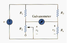
How do we find the current through the galvanometer when the Wheatstone bridge is unbalanced? We find the Thevenin equivalent ( $V_{\text{Th}}$ and $R_{\text{Th}}$) with respect to the galvanometer; the current through it under the unbalanced condition is

$I=\frac{V_{\text{Th}}}{V_{\text{Th}}+R_m}$

SUMMARY

1. A linear network consists of linear elements, linear dependent sources, and linear independent sources.
2. Network theorems are used to reduce a complex circuit to a simpler one, thereby making circuit analysis much simpler.
3. The superposition principle states that for a circuit having multiple independent sources, the voltage across (or current through) an element is equal to the algebraic sum of all the individual voltages (or currents) due to each independent source acting one at a time.
4. Source transformation is a procedure for transforming a voltage source in series with a resistor to a current source in parallel with a resistor or vice versa.
5. Thevenin’s and Norton’s theorems allow us to isolate a portion of a network while the remaining portion of the network is replaced by an equivalent network. The Thevenin equivalent consists of a voltage source $V_{\text{Th}}$ in series with a resistor $R_{\text{Th}}$, while the Norton equivalent consists of a current source $I_N$ in parallel with a resistor $R_N$. The two theorems are related by source transformation.

$R_N=R_{\text{Th}},I_N=\frac{V_{\text{Th}}}{R_{\text{Th}}}$

1. For a given Thevenin equivalent circuit, maximum power transfer occurs when $$$R_L=R_{\text{Th}}$, that is, when the load resistance is equal to the Thevenin resistance.
2. The maximum power transfer theorem states that the maximum power is delivered by a source to the load $R_L$ when the load $R_L$ is equal to $R_{\text{Th}}$, the Thevenin resistance at the terminals of the load.
3. Source modeling and resistance measurement using the Wheatstone bridge provide applications for Thevenin’s theorem.