INTRODUCTION
In sinusoidal circuit analysis, we have learned how to find voltages and currents in a circuit with a constant frequency source. If we left the amplitude of the sinusoidal source remain constant and vary the frequency, we obtain the circuit’s frequency response. The frequency response may be regarded as a complete description of the sinusoidal steady-state behavior of a circuit as a function of frequency.
The frequency response of a circuit is the variation in its behavior with change in signal frequency.
The sinusoidal steady-state frequency responses of circuits are of significance in many applications, especially in communications and control systems. A specific application is in electric filters that block out or eliminate signals with unwanted frequencies and pass signals of the desired frequencies. Filters are used in radio, TV, and telephone systems to separate one broadcast frequency from another.
We begin this chapter by considering the frequency response of simple circuits using their transfer functions. We then consider Bode plots which are the industry-standard way of presenting frequency response. We also consider series and parallel resonant circuits and encounter important concepts such as resonance, quality factor, cutoff frequency and bandwidth. We discuss different kinds of filters and network scaling. In the last section, we consider one practical application of resonant circuits and two applications of filters.
TRANSFER FUNCTION
The transfer function is a useful analytical tool for finding the frequency response of a circuit. In fact, the frequency response of a circuit is the plot of the circuit’s transfer function H( ) versus , with varying from to .
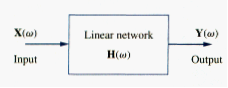
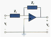
A transfer function is the frequency-dependent ratio of the forced function to the forcing function (or of an output to an input). The idea of a transfer function was implicit when we used the concepts of impedance and admittance to relate voltage and current. In general, a linear network can be represented by the block diagram shown in [link].
The transfer function H( ) of a circuit is the frequency-dependent ratio of a phasor output Y( ) (an element voltage or current) to a phasor input X( ) (source voltage or current).
Thus
assuming zero initial conditions. Since the input and output can be either voltage or current at any place in circuit, there are four possible transfer functions:
where subscripts i and o denote input and output values. Being a complex quantity, H( ) has magnitude H( ) and a phase ; that is .
To obtain the transfer function using [link], we first obtain the frequency-domain equivalent of the circuit by replacing resistors, inductors, and capacitors with their impedances R, j L, and 1/j C. we then use any circuit technique to obtain the appropriate quantity in [link]. We can obtain the frequency response of the circuit by plotting the magnitude and phase of the transfer function as the frequency varies. A computer is a real time-saver for plotting the transfer function.
The transfer function H( ) can be expressed in terms of its numerator polynomial N( ) and denominator polynomial D( ) as
Where N( ) and D( ) are not necessarily the same expressions for the input and output functions, respectively. The representation of H( ) in [link] assumes that common numerator and denominator factors in H( ) have canceled, reducing the ratio to lowest terms. The roots of N( ) = 0 are called the zeros of H( ) and are usually represented as Similarly, the roots of D( ) = 0 are the poles of H( ) and are represented as
A zero as a root of the numerator polynomial, is a value that results in a zero value of the function. A pole, as a root of the denominator polynomial, is a value for which the function is infinite.
To avoid complex algebra, it is expedient to replace j temporarily with s when working with H( ) and replace s with j at the end.
THE DECIBEL SCALE
It is not always easy to get a quick plot of the magnitude and phase of the transfer function as we did above. A more systematic way of obtaining the frequency response is to us Bode plots. Before we begin to construct Bode plots, we should take care of two important issues: the use of logarithms and decibels in expressing gain.
Since Bode plots are based on logarithms, it is important that we keep the following properties of logarithms in mind:
In communications systems, gain is measured in bels. Historically, the bel is used to measure the ratio of two levels of power or power gain G; that is,
The decibel (dB) provides us with a unit of less magnitude. It is of a bel and is given by
When , there is no change in power and the gain is 0 dB. If , the gain is
And when , the gain is
[link] and [link] show another reason why logarithms are greatly used: the logarithm of the reciprocal of a quantity is simply negative the logarithm of that quantity.
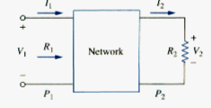
Alternatively, the gain G can be expressed in terms of voltage or current ratio. To do so, consider the network shown in [link]. If is the input power, is the output (load) power, is input resistance and is the load resistance, then and , and [link] becomes
For the case when , a condition that is often assumed when comparing voltage levels, [link] becomes
Instead, if and , for , we obtain
Three things are important to note from [link],[link], and [link]:
- That 10 log is used for power, while 20 log is used for voltage or current, because of the square relationship between them ( ).
- That the dB value is a logarithmic measurement of the ratio of one variable to another of the same type. Therefore, it applies in expressing the transfer function H in [link] and [link], which are dimensionless quantities, but not in expressing H in [link] and [link].
- it is important to note that we only use voltage and current magnitude in [link] and [link]. Negative signs and angles will be handled independently as we will see in section 4.
With this in mind, we now apply the concepts of logarithms and decibels to construct Bode plots.
BODE PLOTS
Obtaining the frequency response from the transfer function as we did in section 2 is an uphill task. The frequency range required in frequency response is often so wide that it is inconvenient to use a linear scale for the frequency axis. Also, there is a more systematic way of locating the important features of the magnitude and phase plots of the transfer function. For these reasons, it has become standard practice to use a logarithmic scale for the frequency axis and a linear scale in each of the separate plots of magnitude and phase. Such semilogarithmic plots of the transfer function-known as Bode plots have become the industry standard.
Bode plots are semilog plots of the magnitude (in decibels) and phase (in degrees) of a transfer function versus frequency.
Bode plots contain the same information as the nonlogarithmic plots discussed in the previous section, but they are much easier to construct, as we shall see shortly.
The transfer function can be written as
Taking the natural logarithm of both sides,
Thus, the real part of ln H is a function of the magnitude while the imaginary part is the phase. In a Bode magnitude plot, the gain
is plotted in decibels (dB) versus frequency. [link] provides a few values of H with the corresponding values in decibels. In a Bode phase plot, is plotted in degrees versus frequency. Both magnitude and phase plots are made on semilog graph paper.
| Magnitude H | 20 (dB) |
| 0.001 | -60 |
| 0.01 | -40 |
| 0.1 | -20 |
| 0.5 | -6 |
| -3 | |
| 1 | 0 |
| 3 | |
| 2 | 6 |
| 10 | 20 |
| 20 | 26 |
| 100 | 40 |
| 1000 | 60 |
A transfer function in the form of [link] may be written in terms of factors that have real and imaginary parts. One such representation might be
which is obtained by dividing out the poles and zeros in H( ). The representation of H( ) as in [link] is called the standard form. In this particular case, H( ) has seven different factors that can appear in various combination in a transfer function. These are:
- A gain K
- A pole or zero (j ) at the origin
- a simple pole or zero
In constructing a Bode plot, we plot each factor separately and then combine them graphically. The factors can be considered one at time and then combined additively because of the logarithm that makes Bode plots powerful engineering tool.
We will now make straight-line plots of the factors listed above. We shall find that these straight-line plots known as Bode plots approximate the actual plots to a surprising degree of accuracy.
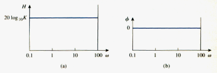
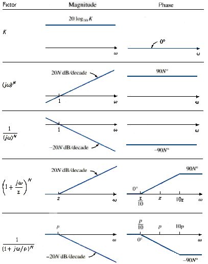
Constant term: for the gain K, the magnitude is 20 K and the phase is 00; both are constant with frequency. Thus, the magnitude and phase plots of the gain are shown in [link]. If K is negative, the magnitude remains 20 but the phase is .
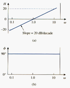
Pole/zero at the origin: for the zero (j ) at the origin, the amplitude is 20 and the phase is 900. These are plotted in [link], where we notice that the slope of the magnitude plot is 20 dB/decade, while the phase is constant with frequency.
The Bode plots for the pole are similar except that the slope of the magnitude plot is -20 dB/decade while the phase is . In general, for is an integer, the magnitude plot will have a slope of 20N dB/decade, while the phase is 90N degrees.
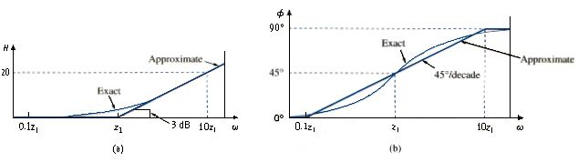
Simple pole/zero: for the simple zero , the magnitude is and the phase is . We notice that
showing that we can approximate the magnitude as zero (a straight line with zero slope) for small values of and by a straight line with slope 20 dB/decade for large values of . The frequency where the two asymptotic lines meet is called the corner frequency or break frequency. Thus, the approximate magnitude plot is shown in [link]a, where the actual plot is also shown. Notice that the approximate plot is close to actual plot except at the break frequency, where and deviation is .
As a straight-line approximation, we let for , for , and for . As shown in [link]b along with the actual plot, the straight-line plot has a slope of per decade.
The Bode plots for the pole are similar to those in [link] except that the corner frequency is at , the magnitude has a slope of – 20 dB/decade, and the phase has a slope per decade
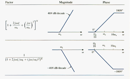
Quadric pole/zero: the magnitude of the quadric pole is and the phase is . But
and
Thus, the amplitude plot consists of two straight asymptotic lines: one with zero slope for and the other with slope -40dB/decade for , with as the corner frequency. [link]a shows the approximate and actual amplitude plots. Note that the actual plot depends on the damping factor as well as the corner frequency . the significant peaking in the neighborhood of the corner frequency should be added to the straight-line approximation if a high level of accuracy is desired. However, we will use the straight-line approximation for the sake of simplicity.
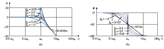
The phase plot is a straight line with a slope of per decade starting at and ending at , as shown in [link]b. We see again that the difference between the actual plot and the straight-line plot is due to the damping factor. Notice that the straight-line approximations for both magnitude and phase plots for the quadratic pole are the same as those for a double pole, i.e. . We should expect this because the double pole equals the quadrate pole when . Thus, the quadratic pole can be treated as a double pole as fa as straight-line approximation is concerned.
For the quadratic zero , the plots in [link] are inverted because the magnitude plot has a slope of 40 dB/decade while the phase plot has a slope of per decade.
[link] presents a summary of Bode plots for the seven factors. To sketch the Bode plots for a function H( ) in the form of [link], for example, we first record the corner frequencies on the semilog graph paper, sketch the factors one at a time as discussed above, and then combine additively the graphs of the factors. The combined graph is often drawn from left to right, changing slopes appropriately each time a corner frequency is encountered.
Summary of Bode straight-line magnitude and phase plots.
SERIES RESPONSE
The most prominent feature of frequency response of a circuit may be the sharp peak (or resonant peak) exhibited in its amplitude characteristic. The concept of resonance applies in several areas of science and engineering. Resonance occurs in any system that has a complex conjugate pair of poles; it is the cause of oscillations of stored energy from one form to another. It is the phenomenon that allows frequency discrimination in communication networks. Resonance occurs in any circuit that has at least one inductor and one capacitor.
esonance is a condition in an RLC circuit in which the capacitive and inductive reactances are equal in magnitude, thereby resulting in a purely reactive impedance.
Resonant circuits (series or parallel) are useful for constructing filters, as their transfer functions can be highly frequency selective. They are used in any applications such as selecting the desired stations in radio and TV receivers.
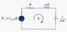
Consider the series RLC circuit shown in [link] in the frequency domain. The input impedance is
or
Resonance results when the imaginary part of the transfer function is zero, or
The value of that satisfies this condition is called the resonant frequency . Thus, the resonance condition is
Or
Since .
Note that at resonance:
1. The impedance is purely resistive, thus, Z = R. in other words, the LC series combination acts like a short circuit, and the entire voltage is across R.
2. The voltage and the current I are in phase, so that the power factor is unity.
3. The magnitude of the transfer function H( ) = Z( ) is minimum.
4. The inductor voltage and capacitor voltage can be much more than the source voltage.
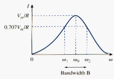
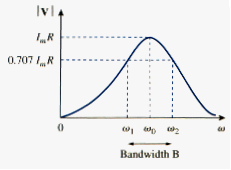
The frequency response of circuit’s current magnitude
Is shown in [link]; the plot only shows the symmetry illustrated in this graph when the frequency axis is a logarithm. The average power dissipated by the RLC circuit is
The highest power dissipated occurs at resonance, when , so that
At certain frequencies , the dissipated power is the half the maximum value; that is,
Hence, and are called the half-power frequencies.
The half-power frequencies are obtained by setting Z equal to and writing
Solving for , we obtain
We can relate the half-power frequencies with the resonant frequency. From [link] and [link],
Solving that the resonant frequency is the geometric mean of the half-power frequencies. Note that and are in general not symmetrical around resonant frequency , because the frequency response is not generally symmetrical. However, as will be explained shortly, symmetry of the half-power frequencies around the resonant frequency is often a reasonable approximation.
Although the height of the curve in [link] is determined by R, the width of the curve depends on other factors. The width of response curve depends on the bandwidth B, which is defined as the difference between the two half-power frequencies,
This definition of bandwidth is just one of several that are commonly used. Strickly speaking, B in[link] is a half-power bandwidth, because it is the width of the frequency band between the half-power frequencies.
The “sharpness” of the resonance in a resonant circuit is measured quantitatively by the quality factor Q. at resonance, the reactive energy in the circuit oscillates between the inductor and the capacitor. The quality factor relates the maximum or peak energy stored to the energy dissipated in the circuit per cycle of oscillation:
Q = 2 __________Peak energy stored in the circuit_____________
Energy dissipated by the circuit in one period at resonance
It is also regarded a measure of the energy storage property of a circuit in relation to its energy dissipation property. In the series RLC circuit, the peak energy stored is , while the energy dissipated in one period is . Hence,
Or
Notice that the quality factor is dimentionless. The relationship between the bandwidth B and the quality factor Q is obtained by substituting [link] into [link] and utilizing [link]
or . Thus
The quality factor of a resonant circuit is the ratio of its resonant frequency to its bandwidth.
Keep in mind that [link], [link], [link], and [link] only apply to a series RLC circuit.
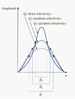
As illustrated in [link], the higher the vale of Q, the more selective the circuit is but the smaller the bandwidth. The selectivity of an RLC circuit is the ability of the circuit to respond to a certain frequency and discriminate against all other frequencies. If the band of frequencies to be selected or rejected is narrow, the quality factor of the resonant circuit must be high. If the band of frequencies is wide, the quality factor must be low.
A resonant circuit is designed to operate at or near its resonant frequency. It is said to be a high-Q circuit when its quality factor is equal to or greater than 10. For high -Q circuits ( ), the half-power frequencies are, for all practical purposes, symmetrical around the resonant frequency and can be approximated as
High-Q circuits are used often in Communications network.
We see that a resonant circuit is characterized by five related parameters: the two half-power frequencies and , the resonant frequency , the bandwidth B, and the quality factor Q.
PARALLEL RESONANCE
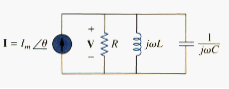
The parallel RLC circuit in [link] is dual of series RLC circuit. So we will avoid needless repetition. The admittance is
Or
Resonance occurs when the imaginary part of Y is zero,
or
which is the same as [link] for the series resonant circuit. The voltage |V| is sketched in [link] as a function of frequency. Notice that at resonance, the parallel LC combination acts like an open circuit, so that the entire current flows through R. also, the inductor and capacitor current can be much more than the source current at resonance.
We exploit the duality between [link] and [link] by comparing [link] with [link]. by replacing R, L, and C in the expressions for the series circuit with 1/R, 1/C, and 1/L respectively, we obtain for the parallel circuit
Using [link] and [link], we can express the half-power frequencies in terms of the quality factor. The result is
Again, for high -Q circuits ( )
[link] presents a summary of the characteristics of the series and parallel resonant circuits.
| Characteristic | Series circuit | Parallel circuit |
| Resonant frequency, | ||
| Quality factor, Q | ||
| Bandwidth, B | ||
| Half-power frequencies | ||
| For , , |
PASSIVE FILTERS
The concept of filters has been an integral part of electrical engineering from the beginning. Several technological achievements would not have been possible without electrical filters. Because of this prominent role of filters, much effort has been expended on the theory, design, and construction of filters and many articles and books have been written on them. Our discussion in this chapter should be considered introductory.
Filter is a circuit that is designed to pass signals with desired frequencies and reject or attenuate others.
As a frequency-selective device, a filter can be used to limit the frequency spectrum of a signal to some specified band of frequencies. Filters are the circuits used in radio and TV receivers to allow us to select one desired signal out of a multitude of broadcast signals in the environment.
A filter is a passive filter if it consists of only passive elements R, L, and C. it is said to be an active filter if it consists of active elements (such as transistors and op amps) in addition to passive elements R, L, and C. we consider passive filters in this section and active filters in the next section. LC filters have been used in practical applications for more than eight decades. LC filter technology feeds related areas such as equalizers, impedance-matching networks, transformers, shaping networks, power dividers, attenuators, and directional couplers, and is continuously providing practicing engineers with opportunities to innovate and experiment. Besides the LC filters we study in these sections, there are other kinds of filters- such as digital filters, electromechanical filters, and microwave filters-which are beyond the level of the text.
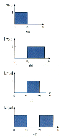
As shown in [link]. There are four types of filters whether passive or active:
- A lowpass filter passes low frequencies and stop high frequencies, as shown ideally in [link]a.
- A high pass filter passes high frequencies and rejects low frequencies, as shown ideally in [link]b.
- A bandpass filter passes frequencies within a frequency band and blocks or attenuates frequencies outside the band, as shown ideally in [link]c.
- A bandstop filter passes frequencies outside a frequency band and blocks or attenuates frequencies within the band, as shown ideally in [link]d.
[link] presents a summary of the characteristics of these filters. Be aware that the characteristics in [link] are only valid for first or second order filters – but one should not have the impression that only these kinds of filter exist. We now consider typical circuits for realizing the filters shown in [link].
| Type of filter | H(0) | H( | H( ) or H( ) |
| Lowpass | 1 | 0 | |
| Highpass | 0 | 1 | |
| Bandpass | 0 | 0 | 1 |
| Bandstop | 1 | 1 | 0 |
Lowpass Filter
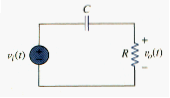
A typical lowpass filter is formed when the output of an RC circuit is taken off the capacitor as shown in [link]. The transfer function is
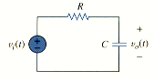
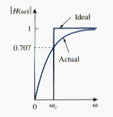
Note that H(0) = 1, H( ) = 0. [link] shows the plot of , along with the ideal characteristic. The half-power frequency, which is equivalent to the corner frequency on the Bode plots but in the context of filters is usually known as the cutoff frequency , is obtained by setting the magnitude of H( ) equal to 1/ , thus
or
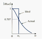
The cutoff frequency is also called the cutoff frequency.
A lowpass filter is designed to pass only frequencies from dc up to the cutoff frequency
A low pass filter can also be formed when the output of an RL circuit is taken off the resistor. Of course, there are many other circuits for lowpass filters.
Highpass Filter
A highpass filter is formed when the output of an RC circuit is taken off the resistor as shown in [link]. The transfer function is
Note that H(0) = 0, H( ) = 1. [link] shows the plot of . Again, the corner or cutoff frequency is
A highpass filter is designed to pass all frequencies above its cutoff frequency .
A highpass filter can also be formed when the output of an RL circuit is taken off the inductor.
Bandpass Filter
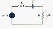
The RLC series resonant circuit provides a bandpass filter when the output is taken off the resistor as shown in [link]. The transfer function is
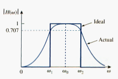
We observe that H(0) = 0, H( ) = 0. [link] shows the plot of . The bandpass filter passes a band of frequency ( ) centered on , the center frequency, which is given by
A bandpass filter is designed to pass all frequencies within a band of frequencies, .
Since bandpass filter in [link] is a series resonant circuit, the half-power frequencies, the bandwidth, and the quality factor are determined as in section 5. A bandpass filter can also be formed by cascading the lowpass filter (where ) in [link] with the highpass filter (where )
Bandstop Filter
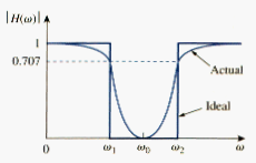
A filter that prevents a band of frequencies between two designated values ( and ) from passing is variably known as a bandstop, bandreject, or notch filter. A bandstop filter is formed when the output RLC series resonant circuit is taken off the LC series combination as shown in [link]. The transfer function is
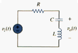
Notice that H(0) = 1, H( ) = 1. [link] shows the plot of . Again, the center frequency is given by
While the half-power frequencies, the bandwidth, and quality factor are calculated using the formulas in section 5 for a series resonant circuit. Here, is called the frequency of rejection, while the corresponding bandwidth ( ) is known as the bandwidth of rejection. Thus,
A bandstop filter is designed to stop or eliminate all frequencies within a band of frequencies, .
Notice that adding the transfer function of the bandpass anf the bandstop gives unity at any frequency for the same values of R, L, and C. Of course, this is not true in general but true for the circuits treated here. This is due to the fact that the characteristic of one is the inverse of the other.
In concluding this section, we should note that:
- From [link], [link], [link], the maximum gain of a passive filter is unity. To generate a gain greater than unity, one should use an active filter as the next section shows.
- There are other ways to get the types of filters treated in this section.
- The filter treated here are the simple types. Many other filters have sharper and complex frequency response.
ACTIVE FILTERS
There are three major limitations to the passive filter in the previous section. First, they cannot generate gain greater than 1; passive elements cannot add energy to the network. Second, they may require bulky and expensive inductor. Third, they perform poorly at frequencies below the audio frequency range (300 Hz < f < 3000 Hz). Nevertheless, passive filters are useful at high frequencies.
Active filters consist of combination of resistors, capacitors, and op amps. They offer some advantage over passive RLC filters. First, they are often smaller and less expensive, because they do not require inductors. This makes feasible the integrated circuit realizations of filters. Second, they can provide amplifier gain in addition to providing the same frequency response as RLC filters. Third, active filter can be combined with buffer amplifiers (voltage followers) to isolate each stage of the filter from source and load impedance effects. This isolation allows designing the stages independently and then cascading them to realize the desired transfer function. (Bode plots, being logarithmic, may be added when transfer function are cascaded.) However, active filters are less reliable and less stable. The practical limit of most active filters is about 100 kHz – most active filters operate well below that frequency.
Filters are often classified according to their order (or number of poles) or their specific design type.
First-Order Lowpass Filter
One type of first-order filter is shown in [link]. The components selected for and determine whether the filter is lowpass or highpass, but one the components must be reactive.
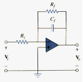
[link] shows a typical active lowpass filter. For this filter the transfer function is
Where and
Therefore,
We notice that [link] is similar to [link], except that there is a low frequency ( ) gain or dc gain of . Also, the corner frequency is
Which does not depend on . This means that several inputs with different could be summer if required, and the corner frequency would remain the same for each input.
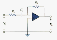
First-Order Highpass Filter
[link] shows a typical highpass filter. As before,
Where and so that
This is similar to [link], except that at very high frequencies ( ), the gain tends to . The corner frequency is
Bandpass Filter
The circuit in [link] may be combined with that in [link] to form a bandpass filter that will have a gain K over the required range of frequencies. By cascading a unit gain lowpass filter, a unit gain highpass filter, and an inverter with gain as shown in the block diagram of [link]a, we can construct a bandpass filter whose frequency response is that in [link]b. The actual construction of the bandpass filter is shown in [link].
The analysis of the bandpass filter is relatively simple. Its transfer function is obtained by multiplying [link] and [link] with the gain of the inverter. That is
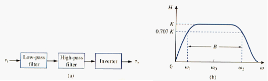
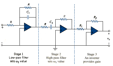
The lowpass section sets upper corner frequency as
While the highpass sets the lower corner frequency as
With these values of and , the center frequency, bandwidth, and quality factor are found as follows:
To find the passband gain K, we write [link] in the standard form of [link],
At the center frequency , the magnitude of the transfer function is
Thus the passband gain is
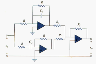
Bandreject (or Notch) Filter
A bandreject filter may be constructed by parallel combination of a low pass filter and a highpass filter and summing amplifier, as shown in the block diagram of [link]a. The circuit is designed such that the lower cutoff frequency is set by the lowpass filter while the upper cutoff frequency is set by the highpass filter. The gap between and is the bandwidth of the filter. As shown in [link]b, the filter passes frequencies below and above . The block diagram in [link]a is actually constructed as shown in [link]. The transfer function is
The formulas for calculating the values of , , the center frequency, bandwidth, and quality factor are the same as in [link] to [link].
To determine the passband gain K of the filter, we can write [link] in terms of the upper and lower corner frequencies as
Comparing this with the standard form in [link] indicates that in the two passbands ( ) and ( ) the gain is
We can also find the gain at the center frequency by finding the magnitude of the transfer function at , writing
Again, the filters treated in this section are only typical. There are many other active filters that are more complex.
SUMMARY
- The transfer function H( ) is the ratio of the output response Y( ) to the input excitation X( ); that is , H( ) = Y( )/X( ).
- The frequency response is the variation of the transfer function with frequency.
- Zeros of a transfer function H(s) are the values of s = j that make H(s) = 0, while poses are the values of s that make .
- The decibel is the unit of logarithmic gain. For a gain G, its decibel equivalent is .
- Bode plots are semilog plots of the magnitude and phase of the transfer function as it varies with frequency. The straight line approximations of H (in dB) and (in degrees) are constructed using the corner frequencies defined by the poles and zeros of H( ).
- The resonant frequency is that frequency at which the imaginary part of a transfer function vanishes. For series and parallel RLC circuits,
- The half-power frequencies ( , ) are those frequencies at which the power dissipated is one-half of that dissipated at the resonant frequency. The geometric mean between the half power frequencies is the resonant frequency, or
- the bandwidth is the frequency band between half-power frequencies:
- The quality factor is a measure of the sharpness of the resonance peak. It is the ratio of the resonant (angular) frequency to the band width,
- A filter is a circuit designed to pass a band of frequencies and reject others. Passive filters are constructed with resistors, capacitors, and inductors. Active filters are constructed with resistors, capacitors, and active devices, usually an op amp.
- Four common types of filters are lowpass, highpass, bandpass, and bandstop. A lowpass filter passes only signals whose frequencies are below the cutoff frequencies . A highpass filter passes only signals whose frequencies are above the cutoff frequency . A bandpass filter passes only signals whose frequecies are within a prescribed range ( ). A bandstop filter passes only signals whose frequencies are outside a prescribed range ( ).