Pham Van Huan
College of Natural Science, Vietnam National University, Hanoi
Abstract: A review of the investigations on the sea level changes in South-china sea is presented and the methods of approximate calculation of theoretical tidal extremes were explained in detail.
The sea level changes near Vietnam coast due to global warming and other effects is evaluated to be from 1 to 3 mm per year.
For seven stations with full set of harmonic constants determined the theoretical extreme heights of tidal level by predicting hourly tide heights in a 20-year period. For other nineteen stations with 11 harmonic constants of main tidal constituents the theoretical astronomical extreme levels were calculated by the iteration method. The comparison showed a good agreement between two methods.
The empirical extreme analysis was carried out for 25 tide gauges along Vietnam coast to evaluate the design values of sea level of different rare frequencies.
The analysis also showed that the tidal extremes and design level values of 20-year return period are of the same range. The level values of longer return period are affected mainly by floods and surges.
1. Introduction
The extreme sea levels are study subject of many purposes. The maximal and minimal values of sea levels and their occurrence probabilities are taken into account in designing hydrotechnical structures.
The theory of extreme analysis of statistical mathematics is applied to the hydrometeorology with different distributions of the observed series of climatic and hydrological parameters [5,7]. The main concepts of these methods will be presented in section 2.1.
In the case that observed series of sea level are not long enough to apply the procedures of extreme analysis theory, that usually happen in the design investigations in the coastal zone and estuaries, one may use theoretical extreme values of purely tidal levels.
In many practical problems the minimal theoretical level is assumed to be the zero depth in tidal seas. This level can be calculated by subtracting maximal low height of tide due to astronomical conditions from mean sea level. In some countries this value is determined by analyzing a predicted series of tidal heights 19-year long, one choose the lowest height among all low waters in the series. In Russia the minimal theoretical level is determined by known method of Vladimirsky.
Vladimirsky method gives an analytical solution of the problem with harmonic constants of 8 main tidal constituents. The rest tidal constituents are taken into account approximately. Recently the calculations can be performed rapidly in computers, evaluating extreme heights of tide can be carried out by more detailed schemes and the accuracy is improved by withdrawing a non-restricted number of tide constituents into consideration [6]. Section 2.2 will explain in details a scheme to implement this method in practice and in section 3 will presented the application results to obtain maximal characteristics of sea level in some region of Vietnam coast.
The observation of sea level along Vietnam coast is mainly carried out by a system of tidal gauges of the Vietnam Hydrometeorological Service. Generally speaking up to now the number of tidal gauges that belongs to Vietnam waters is not many and the number of observation years is not long enough. So there is no much deal with the behavior of sea level in general and the empirical calculations of level extremes in special.
In some rare works there reported the results of analyzing changeableness of sea level and the estimating the trend of sea level rise in the base of analysis of observed series of sea level some years long. The spectrum analysis [2] showed that besides the semiannual and annual periods, in the almost of tidal gauges oscillations of period of 6 to 10 years and longer exist (figure 1).
Table 1 lists the results of estimation of the sea level rise by trend analysis with monthly mean level [2-4]. It is followed that the summary effect by the global warming and oscillations of sea bed in region of Vietnam coast causes a rate of level rise about 13 mm per year.
A full cumbersome calculation of level extremes was performed in [1]. In this report firstly listed series of monthly average, maximal and minimal levels for all gauges along Vietnam coast up to middle of ninetieth. The extreme analysis was carried out by an asymptotic Gumbel function of probability distribution of the extremes.
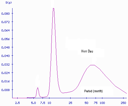
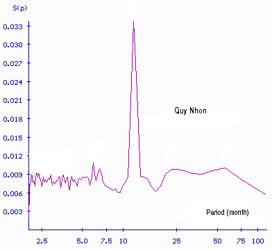
Figure 1. Spectrum of sea level at tidal gauges Hon Dau and Quy Nhon
| Gauge | Co-ordinates | Observation years | Trend (mm/year) |
| Hon Dau | 20°40'N-106°49'E | 1957-1994 | 2,1 |
| Cua Cam | 20°45'N-106°50'E | 1961-1992 | 2,7 |
| Da Nang | 16°06'N-108°13'E | 1978-1994 | 1,2 |
| Quy Nhon | 13°45'N-109°13'E | 1976-1994 | 0,9 |
| Vung Tau | 10°20'N-107°04'E | 1979-1994 | 3,2 |
2. The method of study
2.1. Extremes analysis with empirical data
Assume the values of incidental variable at time and
; .
One is often interest in estimation the probability with which maximal or minimal value exceeds a threshold, or . If the observations on the hydrometeorological parameters are independent and distribute differently due to distribution function , the precise distribution of maximum and minimum can be expressed:
and (1)
The extremes analysis theory says that with the enough length of sample , the probability distribution of the normalized maximum , can be approximated by one of the three following forms of asymptotic function
| (Gumbel function) | ||
| (Frechet function) | (2) | |
| (Weibull function) |
and similarly for the minimal value
| (3) | ||
These different forms of asymptotic functions are dependent to the shape of the trail of probability distribution (the right side for the maxima and the left side for the minima). In practice the sample conditions (the homogeneity, the independence and the dimension) influence on the precision of the approximation by the above asymptotic functions.
Asymptotic extreme distributions include three parameters: shape parameter, local parameter and scale parameter.
Often, instead of estimating the distribution of maxima (or minima), one executes a diverse problem: determine a design value, i. e. a value such as
. (4)
Otherwise is the quantile of extreme distribution. Besides, one converts the probability of the design value to return period , where the time to be expected that threshold is exceeded for the first time, or the average time between two above threshold events.
Using the asymptotic extreme distribution the design values can be easily expressed. For example, with Gumbel distribution, one has:
. (5)
Consequently, design value estimate with return period years of the extreme variable may be calculated knowing parameters and :
, (6)
where is also called "normalized design value".
A question of principle in the application of extremes analysis theory is the precision of the approximation (2) or (3), i. e. the question on the rate of convergence of precise distribution of extremes to the asymptotic one, in practical aspect, the precision of design value estimated by asymptotic distribution in comparison with it's real value (but often unknown) .
The methods of estimation of extreme distribution aim at settlement the question on the initial series, the relatively short length of initial series. Tibor Farago and Richard W. Kats [5] explain different methods to estimate the extreme parameters and determine design values and their estimate accuracy. Section 3.3 presents the results obtained by applying these methods to series of annually maximal and minimal levels of some tidal gauges along Vietnam coast.
2.2. Method of computing extreme values of tide
The tidal height above the mean level may be expressed by the following formula
, (7)
where the reduce coefficients depended on longitude of the rising knot of lunar orbit; the average amplitudes and the phase of tidal constituents.
Depending on the tidal feature, the height of tide may achieve the extremes when longitude of the rising knot of lunar orbit (for diurnal tide) or (for semidiurnal tide). In these conditions ( ) the phases of tidal constituents are expressed through astronomical parameters in table 2.
In table 2 average zone time from midnight; average longitude of the Sun; average longitude of the Moon; average longitude of lunar orbit perigee; special initial phase related to the Greenwich longitude.
The extreme heights of tide may be computed from (7) if the values of astronomical parameters and , which form a combination corresponding to an extreme condition, are known. Investigating on extremes the function from (7), we obtain a system of four equations with four unknowns and whose values determine the extreme condition of the tidal height:
| Tidal constituent | Phase, | |||
| Reduce coefficient, | ||||
| 0,963 | 1,038 | |||
| 1,000 | 1,000 | |||
| 0,963 | 1,037 | |||
| 1,317 | 0,748 | |||
| 1,113 | 0,882 | |||
| 1,183 | 0,806 | |||
| 1,000 | 1,000 | |||
| 1,183 | 0,806 | |||
| 0,928 | 1,077 | |||
| 0,963 | 1,038 | |||
| 0,894 | 1,118 | |||
| 1,000 | 1,000 | |||
| 1,000 | 1,000 |
(8)
where
If the approximate values of astronomical parameters corresponding to extreme condition are known, we may lead equations (8) to a linear form by Taylor expansion. When approximate values of the unknown are sufficiently close to the exact values the expansion can be restricted in first order items.
With designations of corrections to the approximate values of astronomical parameters as following
the result of the expansion is a system of four linear equations with diagonally symmetric coefficient matrix:
, (9)
where
;
phase of the tidal constituents computed through approximate values of the astronomical parameters and
In order to compute the values of astronomical corresponding to extreme condition with a given accuracy the iteration method may be used. If any correction among obtained from solving system (9) exceeds in magnitude a given value the solution will repeated and then in order to compute the coefficients of equations (9) we will use the phases computed through the values corrected of astronomical parameters:
The loop is repeated until all corrections obtained in solution step of system (9) become less than :
.
| Semidiurnal tide | ||||
| Astronomical parameters | Minimal level condition | Maximal level condition | ||
If initial approximate values close to real values the iteration rapidly converges. These values of astronomical parameters corresponding to extreme condition may be calculate through four diurnal or semidiurnal tidal constituents depending on tide feature. The extreme condition for four semidiurnal tidal constituents and diurnal constituents is determined by the following expressions:
- For semidiurnal tide: .
- For diurnal tide: ,
where for the lowest level and for the highest level.
From these expressions follow the formulae for computing the approximate values of astronomical parameters corresponding the extreme conditions (tables 3-6).
In order to compute approximate value of average zone time there are two expressions for the lowest condition and highest condition separately, since for semidiurnal tide one day has two high waters and two low waters. The choice of formula used in concrete case must be reference to the sign of supplementary coefficients and (table 4). Coefficients and are computed by following formulae:
(10)
(11)
| Conditions of the lowest level | Conditions of the highest level |
| when when | when when |
| Diurnal tide | ||
| Astronomical parameters | Conditions of the lowest level | Conditions of the highest level |
The choice of reduce coefficients to compute values is depended on the tide feature:
1) For semidiurnal tide, if then is chosen for ;
2) For diurnal tide, if then is chosen for ;
3) For mixed tide, if then we must use the values of astronomical parameters for both semidiurnal tide (table 3) and diurnal tide (table 5). When compute with astronomical parameters of diurnal tide choose for , when compute with astronomical parameters of semidiurnal tide choose for and . The highest level and the lowest level obtained by three variants will be accepted to be the extremes.
We also compute the approximate values of astronomical parameters corresponding the extreme conditions by Vladimirsky method; this method applied for 8 tide constituents. In Vladimirsky method the extreme heights of tide is determined by consequently choosing values in the interval from 0° to 360°:
(12)
where
The choice of reduce coefficients to compute values is also made as the above recommendations, i. e. with the semidiurnal tide is chosen for , with diurnal tide is chosen for . With mixed tide the computation is performed with for and and than the lowest and highest values in two variants will be the extreme levels.
If compute extreme levels with 8 tide constituents then the last results are obtained directly from the expressions (12). In the case other constituents are taken into the computations, we must reference to values and from analyzing (12) to compute the astronomical parameters corresponding extreme conditions and use them as the approximations to compute the coefficients of equations (9).
The conditions of the lowest level:
and the conditions of the highest level:
where
The last extreme values of tide with arbitrary number of constituents are determined from equation (7) using the values of the astronomical parameters corrected by the iteration method.
However, it is worth to make a note that computation of approximate values of astronomical parameters by formulae in tables 3 and 5 is much simpler than Vladimirsky method when the computation involve more than 8 tide constituents
Thus the procedure of computing extreme levels may be performed due to two following schemes:
1) Regardless what is the number of tidal constituents, due to formulae in tables 3 and 6 determine the approximate values of the astronomical parameters correspondig to extreme conditions, than correct these values by the iteration method. Compute the extreme levels by equation (7).
2) Compute the extreme levels with 8 tidal constituents by Vladimirsky method. If the number of constituents is bigger 8 then compute the approximate values of astronomical parameters of extreme condition for 8 constituents by Vladimirsky method and correct them by the iteration method. Compute the extreme levels by equation (7).
In some cases when shallow water constituents have such a big magnitude that causes the approximate values of astronomical parameters computed by formulae in tables 3 and 5 or by Vladimirsky method insufficiently closed to real values to meet the convergence of the iteration process in solution system (7). If a given number of iteration steps (for example, 8 or 10 steps) do not provide the convergence of the results, one may use the method of consequent approximations.
Each shallow water constituent of big magnitude is decomposed into a number of constituents of the smaller magnitude:
(13)
The number is stated depending on the magnitude of tidal constituents. The solution is performed in some steps, each step include all the calculations to correct the values of astronomical parameters, i. e. forming and solving system (9) and iterative calculations as when to correct the astronomical extreme conditions at a given step. For solving in first step astronomical parameters are computed by the formulae in tables 3 and 5 or by Vladimirsky method; further, their values obtained in each steps are used as initial values for the next step. The magnitude of shallow water constituents is increased from step to step to the full magnitude (for example, in first approximation step the magnitude is chosen as , in second step - , in step - .
3. The results of computing extreme levels in Vietnam coast
3.1. Tidal theoretical extremes for the gauges with full set of harmonic constants
For the hydrographic stations with tidal gauges we had used a series of hourly observed levels of one year duration to compute the full set of harmonic constants (30 constituents or more). The hourly levels were predicted for a period of 20 years (1980-2000). The lowest and highest levels chosen are presented in table 6.
| Station | Co-ordinates | Mean sea level (cm) | |||
| Theoretical extremes (cm) | |||||
| Lowest | Highest | ||||
| Hon Dau | 20°40'N-106°49'E | 185 | -10 | 397 | |
| Cua Gianh | 17°42'N-106°28'E | 107 | -16 | 201 | |
| Da Nang | 16°06'N-108°13'E | 93 | 11 | 175 | |
| Quy Nhon | 13°45'N-109°13'E | 160 | 74 | 248 | |
| Nha Trang | 12°15'5N-109°11'5E | 121 | 8 | 227 | |
| Vung Tau | 10°20'N-107°04'E | 258 | -26 | 412 | |
| Rach Gia | 10°00'N-105°05'E | 5 | -48 | 90 |
3.2. Tidal theoretical extremes computed by iteration method
For the stations with no systematic observation on sea levels we had used series of hourly observed levels of duration of some days to compute harmonic constants of main tidal constituents (by Darwin method or by the least squares method). Than, from these restricted harmonic constants we used the iteration method presented in section 2 to get the extreme characteristics of the tidal levels. The results are written in table 7. In this table are also written the theoretical extremes of tide computed for a period of 20 years to compare. It is showed that for the case of restricted harmonic constants (11 constituents) the results by two computations are the same.
| Station | Mean sea level (cm) | ||||||
| Iteration method | Predicted 20 year period | ||||||
| Lowest | Highest | Lowest | Highest | ||||
| Cua Ong | 2150 | 0 | 472 | 2 | 470 | ||
| Co To | 204 | -10 | 454 | -7 | 454 | ||
| Kien An | 98 | -14 | 215 | -14 | 214 | ||
| Dong Xuyen | 91 | -14 | 206 | -13 | 204 | ||
| Dinh Cu | 58 | -47 | 176 | -46 | 174 | ||
| Kinh Khe | 133 | 57 | 214 | 58 | 214 | ||
| Phu Le | 41 | -97 | 171 | -97 | 169 | ||
| Nhu Tan | 83 | 3 | 166 | 4 | 166 | ||
| Ba Lat | 6 | -108 | 126 | -107 | 125 | ||
| Mui Da | 81 | -64 | 207 | -64 | 206 | ||
| Vam Lau | 30 | -119 | 92 | -117 | 107 |
3.3. Results of computing design levels from observed data
In this section we use series of the yearly minimal and maximal levels at stations to evaluate the design levels with different return periods. In each year one lowest level (or one highest level) was chosen to establish the sample series.
The author of [1] has built the empirical distribution curves by graphical method for 24 stations along Vietnam coast. The results of the investigation showed a good agreement between the empirical distribution curves and the first asymptotic distribution function (Gumbel function). From that there computed the level extremes with rare frequencies.
Table 8 presents an example that we performed by using different methods of evaluation for distribution parameters presented in [5].
The analyzing procedure was carried out for all the stations with the observation of 15 to 35 years long. For each station the design levels were computed by 9 estimating methods. Further, 9 values were averaged (table 9).
Table 8. Example of extremes analysis for station Hon Dau by different methods
| Analysis methods | ||||
| Height (cm) related to return period | ||||
| 20 years | 50 years | 100 years | ||
| Two parameters methods (Gumbel): | ||||
| - Method of moments (theoretical) | 406 | 419 | 428 | |
| - Method of moments (empirical) | 409 | 422 | 432 | |
| - Method of quantiles | 412 | 426 | 436 | |
| - Linear unbiased estimates | 411 | 424 | 435 | |
| - Method of probability - weighted | 418 | 435 | 448 | |
| - Maximum likelihood method | 410 | 424 | 434 | |
| Three parameters methods (Jenkinson): | ||||
| - Method of quantiles | 404 | 413 | 419 | |
| - Method of probability - weighted | 414 | 424 | 434 | |
| - Maximum likelihood method | 404 | 413 | 419 | |
| Average of all methods: | 410 | 422 | 431 |
| N | |||||||||||
| Series member | |||||||||||
| Sorted | Normalized | Probability | Period (years) | N | |||||||
| Series member | |||||||||||
| Sorted | Normalized | Probability | Period (years) | ||||||||
| 1 | 347 | -1,369 | 0,020 | 1,020 | 19 | 377 | 0,449 | 0,528 | 2,120 | ||
| 2 | 349 | -1,112 | 0,048 | 1,050 | 20 | 378 | 0,534 | 0,557 | 2,255 | ||
| 3 | 350 | -0,946 | 0,076 | 1,082 | 21 | 379 | 0,623 | 0,585 | 2,408 | ||
| 4 | 351 | -0,815 | 0,104 | 1,117 | 22 | 379 | 0,715 | 0,613 | 2,584 | ||
| 5 | 351 | -0,703 | 0,133 | 1,153 | 23 | 380 | 0,811 | 0,641 | 2,788 | ||
| 6 | 353 | -0,603 | 0,161 | 1,192 | 24 | 380 | 0,913 | 0,670 | 3,026 | ||
| 7 | 354 | -0,510 | 0,189 | 1,233 | 25 | 382 | 1,022 | 0,698 | 3,309 | ||
| 8 | 362 | -0,423 | 0,217 | 1,278 | 26 | 382 | 1,139 | 0,726 | 3,651 | ||
| 9 | 365 | -0,339 | 0,246 | 1,326 | 27 | 384 | 1,266 | 0,754 | 4,071 | ||
| 10 | 365 | -0,258 | 0,274 | 1,377 | 28 | 386 | 1,406 | 0,783 | 4,600 | ||
| 11 | 366 | -0,180 | 0,302 | 1,433 | 29 | 390 | 1,562 | 0,811 | 5,287 | ||
| 12 | 367 | -0,102 | 0,330 | 1,494 | 30 | 391 | 1,741 | 0,839 | 6,216 | ||
| 13 | 367 | -0,025 | 0,359 | 1,559 | 31 | 395 | 1,950 | 0,867 | 7,540 | ||
| 14 | 368 | 0,052 | 0,387 | 1,631 | 32 | 398 | 2,205 | 0,896 | 9,582 | ||
| 15 | 369 | 0,129 | 0,415 | 1,710 | 33 | 400 | 2,536 | 0,924 | 13,140 | ||
| 16 | 371 | 0,207 | 0,443 | 1,797 | 34 | 400 | 3,015 | 0,952 | 20,901 | ||
| 17 | 371 | 0,286 | 0,472 | 1,893 | 35 | 421 | 3,923 | 0,980 | 51,062 | ||
| 18 | 372 | 0,367 | 0,500 | 2,000 |
| Station | Number of observation years | ||||||||||
| Design levels (cm) related to return period | |||||||||||
| 20 years | 50 years | 100 years | |||||||||
| Highest | Lowest | Highest | Lowest | Highest | Lowest | ||||||
| Cua Ong | 32 | 480 | -2 | 491 | -14 | 499 | -22 | ||||
| Co To | 35 | 467 | -14 | 481 | -25 | 491 | -32 | ||||
| Hon Gai | 31 | 452 | -14 | 464 | -27 | 473 | -37 | ||||
| Cua Cam | 33 | 440 | 17 | 452 | 7 | 460 | -1 | ||||
| Hon Dau | 35 | 410 | -6 | 422 | -14 | 431 | -20 | ||||
| Ba Lat | 33 | 178 | -179 | 192 | -188 | 203 | -194 | ||||
| Hoang Tan | 26 | 284 | -163 | 319 | -170 | 347 | -176 | ||||
| Lach Sung | 25 | 207 | -136 | 230 | -147 | 248 | -155 | ||||
| Cua Hoi | 32 | 221 | -182 | 238 | -194 | 250 | -202 | ||||
| Hon Ngu | 25 | 393 | -7 | 409 | -21 | 421 | -31 | ||||
| Ho Do | 27 | 237 | -132 | 262 | -138 | 281 | -142 | ||||
| Station | Number of observation years | ||||||||||
| Design levels (cm) related to return period | |||||||||||
| 20 years | 50 years | 100 years | |||||||||
| Highest | Lowest | Highest | Lowest | Highest | Lowest | ||||||
| Cam Nhuong | 32 | 242 | -98 | 272 | -104 | 300 | -108 | ||||
| Cua Gianh | 31 | 163 | -148 | 186 | -153 | 204 | -157 | ||||
| Dong Hoi | 33 | 192 | -144 | 217 | -152 | 236 | -158 | ||||
| Cua Viet | 17 | 313 | -1 | 357 | -5 | 396 | -7 | ||||
| Da Nang | 15 | 287 | 9 | 323 | 3 | 349 | -3 | ||||
| Hoi An | 18 | 350 | -34 | 401 | -38 | 441 | -41 | ||||
| Quy Nhon | 16 | 290 | 27 | 299 | 20 | 306 | 15 | ||||
| Phu Quy | 14 | 324 | 64 | 331 | 58 | 335 | 53 | ||||
| Vung Tau | 15 | 434 | -46 | 440 | -55 | 445 | -61 | ||||
| Vam Kinh | 15 | 150 | -325 | 168 | -337 | 182 | -345 | ||||
| Cho Lach | 15 | 202 | -161 | 207 | -168 | 210 | -173 | ||||
| Ca Mau | 16 | 151 | -61 | 168 | -64 | 181 | -67 | ||||
| Phu An | 16 | 152 | -253 | 157 | -264 | 161 | -272 | ||||
| Rach Gia | 16 | 126 | -61 | 136 | -64 | 144 | -66 |
4. Remarks and conclusions
For the stations with restricted set of harmonic constants (less than 11 tide constituents) evaluating theoretical extreme heights of tide by the method of predicting 20-year series of hourly level and by the iteration method gives close to each other results (see table 7).
Note that predicting tide in 20-year period takes great computer time, while the iteration method allows more rapid calculation. Therefore in practical investigation at the region where no gauges set up we should fulfil measure hourly levels in some days to derive the harmonic constants of main tide constituents. Than with the iteration method applied, we can compute the tide theoretical extremes, which have a certain practical usefulness.
The results of analysis showed that the difference between extreme levels in 20-year duration and the design levels of 20-year return period is not bigger than the analysis error in the case of restricted length of used samples.
The theoretical extremes of tide have the sense of extreme levels. For example, in table 6, the lowest level at Hon Dau in period 20 years is -10 cm, the highest is 397 cm. Due to results of evaluating extremes from empirical data the design levels for return period 20 years are -6 vµ 410 cm respectively (table 9). For the return period 50 years and 100 years the pairs of values are (-14; 422) and (-20; 431) respectively. Obviously the lowest levels differ no much, consist of about 10cm. At the same time the highest levels differ from each other up to 30 cm, this reflects the influence of floods and wind surges. However, taking into account the large dispersion of the estimates by different methods, this difference does not exceed the error of estimation. For example, for station Hon Dau, in [1] the estimation by graphical method gives results: for return period 20 years: (-11; 435), 50 years: (-19; 451), 100 years: (-25; 462). With the method of averaging 9 variants that we did, the pairs of values are: for return period 20 years: (-6; 410), 50 years: (-14; 422), 100 years: (-20; 431) (table 9). The differences by now achieve 20 to 30 cm. The difference between variants of estimation may be more substantial with the shorter series. Therefore, the estimation of design levels by different method and averaging results is the best way to provide real design levels in the case of short series.
From the above analysis follows that the obtained here design levels have the different reliability. For the stations with observation more than 30 years the design levels in table 9 can be considered as satisfactory.
References
1. Nguyen Tai Hoi. Report on tidal characteristics (Sub. A5). Design water levels (Sub. A13). Marine Hydrometeorological Centre. Vietnam VA Project, Hanoi, 1995
2. Nghiên cứu sự biến thiên và tương quan của mực nước các trạm dọc bờ Việt Nam và khả năng khôi phục các chuỗi mực nước ở một số trạm quan trắc. Báo cáo thực hiện chuyên đề do Nguyễn Ngọc Thụy, Phạm Văn Huấn, Bùi Đình Khước thực hiện / Đề tài cấp nhà nước KT-03-03, 1995
3. Nguyễn Ngọc Thụy. Về xu thế nước biển dâng ở Việt Nam. Tạp chí Khoa học Kỹ thuật biển, số 1, Hà Nội, 1993
4. Xác định thêm về xu thế mực nước biển tại một số điểm ven bờ biển Việt Nam. Báo cáo thực hiện chuyên đề do Bùi Đình Khước thực hiện / Đề tài cấp nhà nước KT-03-03, 1993
5. Tibor Farago, Richard W. Kats. Extremes and dessign values in climatology. WCAP-14, WMO/TD-No 386, World Meteorological Organization, 1990
6. Пересыпкин В. И. Аналитические методы расчета колебаний уровня моря. Гидрометеоиздат., Ленинград, 1961
7. Руководство по расчету гидрологических характеристик для исследований и изысканий в береговых зонах и эстуариев. Наука, Москва, 1973
MỰC NƯỚC CỰC TRỊ Ở VÙNG BIỂN VIỆT NAM
Phạm Văn Huấn
Trường Đại học Khoa học Tự nhiên - ĐHQGHN
Tóm tắt: Giới thiệu tổng quan những kết quả nghiên cứu về biến thiên mực nước biển ở biển Đông và trình bày chi tiết về các phương pháp tính toán gần đúng các cực trị thuỷ triều lý thuyết.
Biến thiên mực nước biển gần bờ Việt Nam do sự nóng lên toàn cầu và các hiệu ứng khác được ước lượng bằng khoảng từ 1 đến 3 mm một năm.
Với bảy trạm hải văn có bộ hằng số điều hoà thủy triều đầy đủ đã xác định được các độ cao mực triều cực trị bằng cách tính các độ cao mực triều từng giờ trong chu kỳ 20 năm. Với 19 trạm khác có 11 hằng số điều hoà của các phân triều chính, các mực nước cực trị thiên văn lý thuyết được ước lượng bằng phương pháp lặp. So sánh cho thấy hai phương pháp cho kết quả khá phù hợp.
Phép phân tích cực trị thực nghiệm được thực hiện cho 25 trạm mực nước dọc bờ Việt Nam để ước lượng các trị số mực nước thiết kế ứng với các tần xuất hiếm khác nhau.
Phân tích so sánh chỉ ra rằng các cực trị thủy triều và mực nước thiết kế chu kỳ lặp lại 20 năm có độ lớn như nhau. Còn những trị số mực nước thiết kế với chu kỳ lặp lại dài hơn bị ảnh hưởng chủ yếu bởi hiện tượng lũ và nước dâng.
Địa chỉ tác giả: Phạm Văn Huấn, Khoa Khí tượng Thuỷ văn và Hải dương học, Trường ĐHKHTN
Phone: 0912 116661 E-mail: huanpv@fpt.vn