INTRODUCTION
Now that we have considered the three passive elements (resistors, capacitors, and inductors) and one active element (the op amp) individually, we are prepared to consider circuits that contain various combinations of two or three of passive elements. In this chapter, we shall examine two types of simple circuits: a circuit comprising a resistor and capacitor and a circuit comprising a resistor and an inductor. These are called RC and RL circuits, respectively. As simple as these circuits are, they find continual applications in electronics, communications, and control system, as we shall see.
We carry out the analysis of RC and RL circuits by applying Kirchhoff’s laws, as we did for resistive circuits. The only difference is that applying Kirchhoff’s laws to purely resistive circuits, results in algebraic differential equations, which are more difficult to solve than algebraic equations. The differential equations resulting from analyzing RC and RL circuits are of the first order. Hence, the circuits are collectively known as first-order circuits.
A first-order circuit is characterized by a first-order diferential equation.
In addition to there being two types of first-order circuits (RC and RL), there are two ways to excite the circuits. The first way is by called source-free circuits, we assume that energy is initially stored in the capacitive or inductive element. The energy circuit and is gradually dissipated in the resistors. Although source-free circuits are by definition free of independent sources, they may have dependent sources. The second way of exiting first-order circuits is by independent sources. In this chapter, the independent sources we will consider are dc sources. The two types of first-order circuits and the two ways of exiting them and add up to the four possible situations we will study in this chapter.
Finally, we consider four typical applications of RC and RL circuits delay and relay circuits, a photoflash unit, and an automobile ignition circuit.
THE SOURCE-FREE RC CIRCUIT
A source-free RC circuit occurs when its dc source is suddenly disconnected. The energy already stored in the capacitor is released to the resistors.
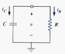
Consider a series combination of a resistor and an initially charged capacitor, as shown in [link]. (The resistor and capacitor may be the equivalent resistance and equivalent capacitance of combination of resistors and capacitors.) Our objective is to determine the circuit response, which, for pedagogic reasons, we assume to be the voltage v(t) across the capacitor. Since the capacitor is initially charged, we can assume that at time t = 0, the initial voltage is
With the corresponding value of the energy stored as
Applying KCL at the top note of the circuit in [link],
By definition, and . Thus,
or
This is a first order differential equation, since only the first derivative of v is involved. To solve it, we arrange the terms as
integrating both sides, we get
where ln A is the integration constant. Thus,
Taking powers of e produces
But from the initial conditions, . Hence,
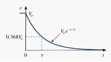
This shows that the voltage response of the RC circuit is an exponential decay of the initial voltage. Since the response is due to the initial energy stored and the physical characteristics of the circuit and not due to some external voltage or current source, it is called the natural response of the circuit.
The natural response of a circuit refers to the behavior (in terms of voltages and currents) of the circuit itself, with no external sources of excitation.
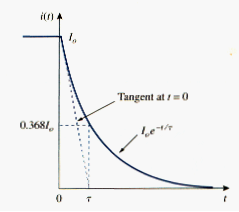
The natural response is illustrated graphically in [link]. Note that at t = 0, we have the correct initial condition as in [link]. as t increases, the voltage decreases toward zero. The rapidity with which the voltage decreases is expressed in terms of the time constant, denoted by , the lower case greek letter tau.
The time constant of a circuit is the time required for the response to decay by a factor of 1/e or 36.6 percent of its initial value.
This implies that at , [link] becomes
or
In terms of the time constant, [link] can be written as
With a calculator it is easy to show that the value of is as shown in [link]. It is evident from [link] that the voltage v(t) is less than 1 percent of after 5 (five time constants). Thus, it is customary to assume that the capacitor is fully discharged (or charged) after five time constants. In other words, it takes 5 for the circuit to reach its final for every time interval of , the voltage is reduced by 36.8 percent of its previous value, , regardless of the value of t.
Values of
| t | |
| 0.36788 | |
| 2 | 0.13534 |
| 3 | 0.04979 |
| 4 | 0.01832 |
| 5 | 0.00674 |
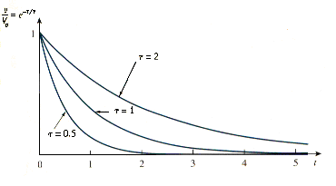
Observe from [link] that the smaller the time constant, the more rapidly the voltage decreases, that is, the faster the response. This is illustrated in [link]. A circuit with a small time constant gives a fast response in that it reaches the steady state (or final state) quickly due to quick dissipation of energy stored, whereas a circuit with a large time constant gives a slow response because it takes longer to reach steady state. At any rate, whether the time constant is small or large, the circuit reaches steady state in five time constants.
With the voltage v(t) in [link], we can find the current ,
The power dissipated in the resistor is
The energy absorbed by the resistor up to time t is
Note that as , , which is the same as , the energy initially stored in the capacitor. The energy that was initially stored in the capacitor is eventually dissipated in the resistor.
In summary:
The key to working with a source-free RC circuit is finding:
- The initial voltage across the capacitor.
The time constant .
With these two items, we obtain the response as the capacitor voltage . Once the capacitor voltage is first obtained, other variables (capacitor current iC, resistor voltage , and resistor current ) can be determined. In finding the time constant , R is often the Thevenin equivalent resistance at the terminals of the capacitor; that is, we take out the capacitor C and find at its terminals.
THE SOURCE-FREE RL CIRCUIT
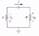
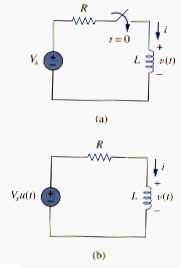
Consider the series connection of a resistor and inductor, as shown in [link]. Our goal is to determine the circuit response, which we will assume to be the current i(t) through the inductor. We select the inductor current as the response in order to take advantage of the idea that the inductor current can not change instantaneously. At t = 0, we assume that the inductor has an initial current I0, or
With the corresponding energy stored in the inductor as
Applying KVL around loop in [link],
But and . Thus,
Or
Rearranging terms and integrating gives
or
Taking the powers of e, we have
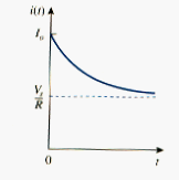
This shows that the natural response of the RL circuit is an exponential decay of the initial current. The current response is shown in [link]. It is evident from [link] that the time constant for the RL circuit is
with again having the unit of seconds. Thus, [link] may be written as
With the current in [link], we can find the voltage across the resistor as
The power dissipated in the resistor is
The energy absorbed by the resistor is
or
Note that as , , which is the same as , the initial energy stored in the inductor as in [link]. Again, the energy initially stored in the inductor is eventually dissipated in the resistor.
In summary:
The key to working with a source-free RL circuit is to find:
- The initial current through the inductor.
The time constant of the circuit.
With the two terms, we obtain the response as the inductor current . Once we determine the inductor current , other variables (inductor voltage , resistor voltage , and resistor current ) can be obtained. Note that in general, R in [link] is the Thevenin resistance at the terminals of the inductor.
SINGULARITY FUNCTIONS
Before going on with the second half of this chapter, we need to digress and consider some mathematical concepts that will aid our understanding of transient analysis. A basic understanding of singularity functions will help us make sense of the response of first-order circuits to a sudden application of an independent dc voltage or current source.
Singularity functions (also called switching functions) are very useful in circuit analysis. They serve as good approximations to the switching signals that arise in circuits with switching operations. They are helpful in the neat, compact description of some circuit phenomena, especially the step response of RC or RL, circuits to be discussed in the next sections. By definition,
Singularity functions are functions that either are discontinuous or have discontinuous derivatives.
The three most widely used singularity functions in circuit analysis are the unit step, the unit impulse, and the unit ramp functions.
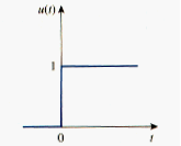
The unit step function u(t) is 0 for negative values of t and 1 for positive values of t.
The unit step function is undefined at t = 0, where it changes abruptly from 0 to 1. It is dimensionless, like other mathematical functions, such as sine and cosine. [link] depicts the unit step function.
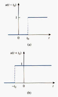
It is the same as saying that u(t) is delayed by seconds, as shown in [link], we simply replace every t by .
u(t) is advanced by seconds, as shown in [link]b.
We use the step function to represent an abrupt change in voltage or current, like the changes that occur in the circuits of control systems and digital computers.
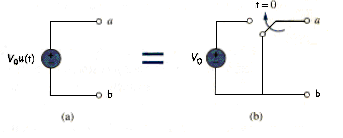
We may express in terms of the unit step function as
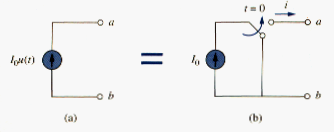
If we let , then v(t) is simply the step voltage . A voltage source of is shown in [link](a); its equivalent circuit is shown in [link](b). It is evident in [link](b) that terminals a-b are short circuited (v = 0) for t < 0 and that appears at the terminals for t > 0. Similarly, a current source of is shown in [link](a), while its equivalent circuit is in [link](b). Notice that for t < 0, there is an open circuit (i = 0), and that flows for t > 0.
The derivative of the unit step function u(t) is the unit impulse function .
The unit impulse function - also known as the delta function - is shown in [link].
The unit impulse function is zero everywhere except at t = 0, where it is undefined.
Impulsive currents and voltages occur in electric circuits as a result of switching operations or impulsive sources. Although the unit impulsive function is not physically realizable (just like ideal sources, ideal resistors etc.), it is a very useful mathematical tool.
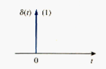
The unit impulse may be regarded as an applied or resulting shock. It may be visualized as a very short duration pulse of unit area. This may be expressed mathematically as
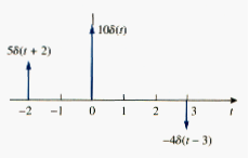
Where denotes the time just before t = 0 and is the time just after t = 0. For this reason, it is customary to write 1 (denoting unit area) beside the arrow that is used to symbolize the unit impulse function. When an impulse function has a strength other than unity, the area of the impulse is equal to its strength. For example, an impulse function 10 has an area of 10. [link] shows the impulse functions , 10 , and .
To illustrate how the impulse function effects to other functions, let us evaluate the integral
where . Since except , the integrand is zero except at . Thus,
Or
This shows that when a function is integrated with the impulse function, we obtain the value of the function at the point where the impulse occurs. This is a highly useful property of the impulse function known as the sampling or sifting property. The special case of [link] is for . Then [link] becomes
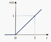
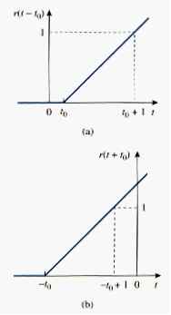
Integrating the unit step function u(t) results in the unit ramp function r(t); we write
The unit ramp function is zero for negative values of t and has a unit slope for positive values of t.
[link] shows the unit ramp function. In general, a ramp is a function that changes at a constant rate.
The unit ramp function may be delayed or advanced as shown in [link].
We should keep in mind that the three singularity functions (impulse, step, and ramp) are related by differentiation as
or by integration as
although there are many more singularity functions, we are only interested in these three (the impulse function, the unit step function, and the ramp function) at this point.
STEP RESPONSE OF AN RC CIRCUIT
When the dc source of an RC circuit is suddenly applied, the voltage or current source can be modeled as a step function, and the response is known as a step response.
The step response of a circuit is its behavior when the excitation is the step function, which may be a voltage or a current source.
The step response is the response of the circuit due to a sudden application of a dc voltage or current source.
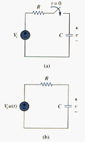
Consider RC circuit in [link](a) which can be replaced by the circuit in [link](b), where is a constant, dc voltage source. Again, we select the capacitor voltage as the circuit response to be determined. We assume an initial voltage on the capacitor, although this is not necessary for the step response. Since the voltage of a capacitor cannot change instantaneously,
where is voltage across the capacitor just before switching and is its voltage immediately after switching. Applying KCL, we have
or
where v is the voltage across the capacitor. For t > 0, [link] becomes
Rearranging terms gives
or
Integrating both sides and introducing the initial conditions,
Or
Taking the exponential of both sides
or
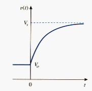
This is known as the complete response (or total response) of the RC circuit to a sudden application of a dc voltage source, assuming the capacitor is initially charged. The reason for the term “complete” will become evident a little later. Assuming that , a plot of is shown in [link].
If we assume that the capacitor is uncharged initially, we set in [link].
We can write alternatively as
this is the complete step response of the RC circuit when the capacitor is initially uncharged. The current through the capacitor is obtained from [link] using . We get
or
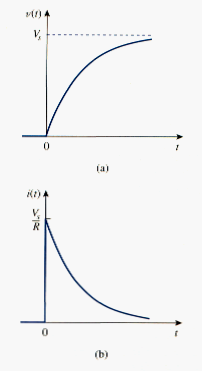
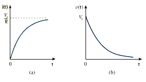
[link] shows the plot of capacitor voltage v(t) and capacitor current i(t).
Rather than going through the derivations above, there is a systematic approach – or rather, a short-cut method – for finding the step response of RC or RL circuit. Let us reexamine [link], which is more general than [link]. It is evident that v(t) has two components.
Classically there are two ways of decomposing this into two components. The first is to break it into a “natural response and a forced response” and the second is to break it into a “transient response and a steady-state response”. Starting with natural response and forced response, we write the total or complete response as
Complete response = Natural response (stored energy) + Forced response (independent source)
or
Where
and
we are familiar with the natural response of the circuit, as discussed in section 2, is known as forced response because it is produced by the circuit when an external “force” (a voltage source in this case) is applied. It represents what the circuit is forced to do by the input excitation. The natural response eventually dies out along with the transient component of the forced response, leaving only the steady-state component of the forced response.
Another way of looking at the complete response is to break into two components – one temporary and the other permanent, i.e.
Complete response = Transient response (temporary part) + Steady –state response (permanent part)
or
where
and
The transient response is temporary; it is the portion of the complete response that decays to zero as time approaches infinity. Thus,
The transient response is the circuit’s temporary response that will die out with time.
The steady-state response is portion of the complete response that remains after the transient response has died out . Thus,
The steady-state response is the behavior of circuit a long time after an external excitation is applied.
The first decomposition of the complete response is in terms of the source of the responses, while the second decomposition is in term of the permanency of the responses. Under certain conditions, the natural response and transient response are the same. The same can be said about the forced response and the steady-state response.
Whichever way we look at it, the complete response in [link] may be written as
where v(0) is the initial voltage at and is the final steady-state value. Thus, to find the step response of an RC circuit requires three things:
- The initial capacitor voltage v(0),
- The final capacitor voltage ,
- The time constant ,
We obtain item 1 from the given circuit for t < 0 and items 2 and 3 from the circuit for t > 0. Once these items are determined, we obtain the response using [link]. This technique equally applies to RL circuits, as we shall see in the next section.
Note that if the switch changes position at time instead of at t = 0, there is a time delay in the response so that becomes
where is initial value at . Keep in mind that [link] or [link] applies only to step response, that is, when the input excitation is constant.
STEP RESPONSE OF AN RL CIRCUIT
Consider the RL circuit in [link](a), which may be replaced by the circuit in [link](b). Again, our goal is to find the inductor current i as the circuit response. Rather than apply Kirchhoff’s laws, we will use the simple technique in [link] through [link]. Let the response be the sum of the natural current and the forced current,
We know that the natural response is always a decaying exponential, that is,
and
where A is a constant to be determined.
The forced response is the value of the current a long time after the switch in [link](a) is closed. We know that the natural response essentially dies out after five time constants. At that time, the inductor becomes a short circuit, and the voltage across it is zero. The entire source voltage V, appears across R. Thus, the forced response is
Substituting [link] and [link] into [link] gives
We now determine the constant A from the initial value of i. Let be the initial current through the inductor, which may come from a source other than . since the current through the inductor cannot change instantaneously,
Thus at t = 0, [link] becomes
From this, we obtain A as
Substituting for A in [link], we get
This is complete response of the RL circuit. It is illustrated in [link]. The response in [link] may be written as
Where i(0) and are the initial and final values of i. Thus, to find the step response of an RL, circuit requires three things:
- The initial the inductor current i(0) at ,
- The final inductor current
- The time constant
We obtain 1 from the given circuit for t < 0 and items 2 and 3 from the circuit for t > 0. Once these items are determined, we obtain the response using [link]. Keep in mind that this technique applies only for step responses.
Again, if the switching takes place at time , instead of t = 0, [link] becomes
If , then
This is the step response of the RL circuit with no initial inductor current. The voltage across the inductor is obtained from [link] using . We get
or
[link] shows the step response in [link] and [link].
SUMMARY
- The analysis in this chapter is applicable to any circuit that can be reduced to an equivalent circuit comprising a resistor and a single energy storage element (inductor or capacitor). Such a circuit is the first-order because its behavior is described by a first-order differential equation. When analyzing RC and RL circuits, one must always keep in mind that the capacitor is an open circuit to steady-state dc conditions while the inductor is a short circuit to steady-state dc conditions.
- The natural response is obtained when no independent source is present. It has the general form
where x represents current through (or voltage across) a resistor, a capacitor, or an inductor, and x(0) is the initial value of x. because most practical always have losses, the natural response is a transient response, i.e. it dies out with time.
- The time constant τ is the time required for a response to decay to 1/e of its initial value. For RC circuits, τ = RC and for RL circuits, .
- The singularity functions include the unit step, the unit ramp function, and the unit impulse functions.
The unit impulse function is
- The steady-state response is the behavior of the circuit after an independent source has been applied for a long time. The transient response is the component of the complete response that dies out with time.
- The total or complete response consists of the steady-state response and the transient response.
- The step response is the response of the circuit to a sudden application of a dc current or voltage. Finding the step response of a first-order circuit requires the initial value , the final value , and the time constant . with these three items, we obtain the step response as
A more general form of this equation is
Instantaneous value = final + {initial – final} .