INTRODUCTION

In previous chapter we considered circuits with a single storage element (a capacitor or an inductor). Such circuits are first-order because the differential equations describing them are first-order. In this chapter we will consider circuits containing two storage elements. These are known as second order circuits because their responses are described by differential equations that contain second derivatives.

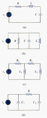
Typical examples of second-order circuits are RLC circuits, in which the three kinds of passive elements are present. Examples of such circuits are shown in [link](a) and [link](b). Other examples are RC and RL circuits, as shown in [link](c) and [link](d). It is apparent from [link] that a second-order circuit may have two storage elements of different type or the same type (provided elements of the same type cannot be represented by an equivalent single element). An op amp circuit with two storage elements may also be a second-order circuit. As with first-order circuits, a second-order circuit may contain several resistors and dependent and independent sources.

A second-order circuit is characterized by a second-order differential equation. It consists of resistors and the equivalent of two energy storage elements.

Our analysis of second-order circuits will be similar to that used for first-order. We will first consider circuits that are excited by the initial conditions of the storage elements. Although these circuits may contain dependent sources, they are free of independent sources. These source-free circuits will give natural responses as expected. Later we will consider circuits that are excited by independent sources. These circuits will give both the transient response and the steady-state response. We consider only dc independent sources in this chapter.

We begin by learning how to obtain the initial conditions for the circuit variables and their derivatives, as this is crucial to analyzing second-order circuits. Then we consider series and parallel RLC circuits such as shown in Fig 1 for the two cases of excitation: by initial conditions of the energy storage elements and by step inputs. Later we examine other types of second-order circuits.

THE SOURCE-FREE SERIES RLC CIRCUIT

An understanding of the natural response of the series RLC circuit is a necessary background for future studies in filter design and communications networks.

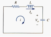
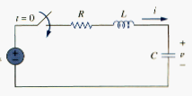
Consider the series RLC circuit shown in [link]. The circuit is being excited by the energy initially stored in the capacitor and inductor. The energy is represented by the initial capacitor voltage V0 and initial inductor current I0. Thus, at t = 0,

Applying KVL around the loop in [link],

To eliminate the integral, we differentiate with respect to t and rearrange terms. We get

This is a second-order differential equation and is the reason for calling the RLC circuits in this chapter second-order circuits. Our goal is to solve [link]. To solve such a second-order differential equation requires that we have two initial conditions, such as the initial value of i and its first derivative or initial values of some i and v. The initial value of i is given in [link]. We get the initial value of the derivative of I from [link] and [link]; that is,

$\text{Ri}(0)+L\frac{\text{di}(0)}{\text{dt}}+V_0=0$

Or

with the two initial conditions in [link] and [link], we can now solve [link]. Our experience in the preceding chapter on first-order circuits suggests that the solution is of exponential form. So we let

where A and s are constants to be determined. Substituting [link] into [link] and carrying out the necessary differentiations, we obtain

${\text{As}}^2{e}^{\text{st}}+\frac{\text{AR}}{L}{\text{se}}^{\text{st}}+\frac{A}{\text{LC}}{e}^{\text{st}}=0$

Or

Since $i={\text{Ae}}^{\text{st}}$ is assumed solution we are trying to find, only the expression in parentheses can be zero:

This quadratic equation is known as the characteristic equation of the differential [link], since the roots of the equation dictate the character of i. The two roots of [link] are

A more compact way of expressing the roots is

Where

The roots s1 and s2 are called natural frequencies, measured in nepers per second (Np/s), because they are associated with the natural response of the circuit; ω0 is known as the resonant frequency or strictly as the undamped natural frequency or the damping factor, expressed in nepers per second. In terms of α and ω0, [link] can be written as

The variables s and ${\omega }_0$ are important quantities we will be discussing throughout the rest of the text.

The two values of s in [link] indicate that there are two possible solutions for I, each of which is of the form of the assumed solution in [link]; that is,

and

$i_2=A{}_2{e}^{s_{2}t}$

Since [link] is a linear equation, any linear combination of the two distinct solutions i1 and i2 is also a solution of [link]. A complete or total solution of [link] would therefore require a linear combination of $i_1$ and $i_2$. Thus, the natural response of the series RLC circuit is

Where the constants A1 and A2 are determined from the initial values i(0) and di(0)/dt in [link] and [link].

From [link], we can infer that there are three types of solutions:

1. If $\alpha >{\omega }_0$, we have the overdamped case.

2. If $\alpha ={\omega }_0$, we have the critically damped case.

3. If , we have the underdamped case.

We will consider each of these cases separately.

Overdamped case ( $\alpha >{\omega }_0$)

From [link] and [link], $\alpha >{\omega }_0$ implies $C>\mathrm{4L}/R^2$. When this happens, both roots $s_1$ and $s_2$ are negative and real. The response is

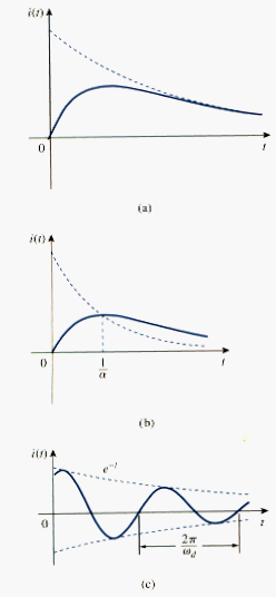
which decays and approaches zero as t increases. [link](a) illustrates a typical overdamped response.

Critically damped case ( $\alpha ={\omega }_0$)

When $\alpha ={\omega }_0$, $C=\mathrm{4L}/R^2$ and

For this case, [link] yields

$i(t)=A_1{e}^{-\mathrm{\alpha t}}+A_2{e}^{-\mathrm{\alpha t}}=A_3{e}^{-\mathrm{\alpha t}}$

Where $A_3=A_1+A_2$. This cannot be the solution, because the two initial conditions cannot be satisfied with single constant. What then could be wrong? Our assumption of an exponential solution is incorrect for the special case of critical damping. Let us go back to [link]. When $\alpha ={\omega }_0=R/\mathrm{2L}$, [link] becomes

$\frac{d^{2}i}{{\text{dt}}^2}+\mathrm{2\alpha }\frac{\text{di}}{\text{dt}}+{\alpha }^{2}i=0$

or

If we let

then [link] becomes

$\frac{\text{df}}{\text{dt}}+\mathrm{\alpha f}=0$

which is a first-order differential equation with solution $f=A_1{e}^{-\mathrm{\alpha t}}$, where $A_1$ is a constant. [link] then becomes

$e^{\mathrm{\alpha t}}\frac{\text{di}}{\text{dt}}+e^{\mathrm{\alpha t}}\mathrm{\alpha i}=A{}_1$

or

This can be written as

Integrating both sides yields

$e^{\mathrm{\alpha t}}i=A_{1}t+A_2$

or

where $A_2$ is another constant. Hence, the natural response of the critically damped circuit is a sum of two terms: a negative exponential and a negative exponential multiplied by a linear term, or

A typical critically damped response is shown in [link](b). In fact, [link](b) is a sketch of $i(t)={\text{te}}^{-\mathrm{\alpha t}}$, which reaches a maximum value of $e^{-1}/\alpha$ at $t=1/\alpha$, one time constant, and the decays all the way to zero.

Underdamped case ( )

For , . The roots may be written as

Where $j=\sqrt{-1}$and ${\omega }_d=\sqrt{{\omega }_0^2-{\alpha }^2}$, which is called the damping frequency. Both ${\omega }_0$ and ${\omega }_d$ are natural frequencies because they help determine the natural response; while

${\omega }_0$ is often called the undamped natural frequency, ${\omega }_d$ is called the damped natural frequency. The natural response is

Using Euler’s identities,

We get

Replacing constants $(A_1+A_2)$ and $j(A_1-A_2)$ with constants $B_1$ and $B_2$, we write

With the presence of sine and cosine functions, it is clear that the natural response for this case is exponentially damped and oscillatory in nature. The response has a time constant of $1/\alpha$ and a period of $T=\mathrm{2\pi }/{\omega }_d$. [link](c) depicts a typical underdamped response. [link] assumes for each case that i(0) = 0.

Once the inductor current i(t) is found for RLC series circuits as shown above, other circuit quantities such as individual element voltages can easily be found. For example, the resistor voltage is $v_R=\text{Ri}$, and the inductor voltage is $v_L=L\text{di}/\text{dt}$. The inductor current i(t) is selected as the key variable to be determined first in order to take advantage of [link].

We conclude this section by noting the following interesting, peculiar properties of an RLC network:

1. The behavior of such a network is captured by the idea of damping, which is the gradual loss of the initial stored energy, as evidenced by the continuous decrease in the amplitude of the response. The damping effect is due to the presence of the resistance R. The damping factor  determines the rate at which the response is damped. If R = 0, then $\alpha =0$, and we have an LC circuit with $1/\sqrt{\text{LC}}$as the undamped natural frequency. Since in this case, the response is not only undamped but also oscillatory. The circuit is said to be lossless, because dissipating or damping element (R) is absent. By adjusting the value of R, the response may be made undamped, overdamped, critically damped, or underdamped.

2. Oscillatory response is possible due to the presence of the two types of storage elements. Having both L and C allows the flow of energy back and forth between the two. The damped oscillation exhibited by the underdamped response is known as ringing. It stems from the ability of the storage elements L and C to transfer energy back and forth between them.

3. Observe from [link] that the waveforms of the responses differ. In general, it is difficult to tell from the waveforms the difference between the overdamped and critically damped responses. The critically damped case is the borderline between the underdamped and overdamped cases and it decays the fastest. With the same initial conditions, the overdamped case has the longest settling time, because it takes the longest time to dissipate the initial stored energy. If we desire the the fastest response without oscillation or ringing, the critically damped circuit is right choice.

THE SOURCE-FREE PARALLEL RLC CIRCUIT

Parallel RLC circuits find many practical applications, notably in communications networks and filter designs.

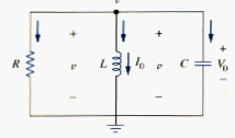
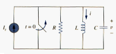
Consider the parallel RLC circuit shown in [link]. Assume initial inductor current I0 and initial capacitor voltage V0,

Since the three elements are in parallel, they have the same voltage v across them. According to passive sign convention, the current is entering each element; that is, the current through each element is leaving the top node. Thus, applying KCL at the top node gives

Taking the derivative with respect to t and dividing by C results in

We obtain the characteristic equation by replacing the first derivative by s and the second derivative by $s^2\frac{}{}\frac{}{}$ . By following the same reasoning used in establishing [link] through [link], the characteristic equation is obtained as

The roots of the characteristic equations are

$s_{\mathrm{1,2}}=-\frac{1}{2\text{RC}}\pm \sqrt{(\frac{1}{2\text{RC}}{)}^2-\frac{1}{\text{LC}}}$

Or

Where

The names of these terms remain the same as in the preceding section, as they play the same role in the solution. Again, there are three possible solutions, depending on whether $\alpha >{\omega }_0$, $\alpha ={\omega }_0$, or . Let us consider these cases separately.

Overdamped case ( $\alpha >{\omega }_0$)

From [link], $\alpha >{\omega }_0$ when $L>{\mathrm{4R}}^{2}C$. The roots of characteristic equation are real and negative. The response is

Critically damped case ( $\alpha ={\omega }_0$)

For $\alpha ={\omega }_0$, $L={\mathrm{4R}}^{2}C$. The roots are real and equal so that the response is

Underdamped case ( )

When , . In this case the roots are complex and may be expressed as

Where

The response is

The constants A1 and A2 in each case can be determined from the initial conditions. We need v(0) and dv(0)/dt. The first term is known from [link]. We find the second term by combining [link] and [link], as

$\frac{V_0}{R}+I_0+C\frac{\text{dv}(0)}{\text{dt}}=0$

Or

The voltage waveforms are similar to those shown in [link] and will depend on whether the circuit is overdamped, underdamped, or critically damped.

Having found the capacitor voltage v(t) for the parallel RLC circuit as shown above, we can readily obtain other circuit quantities such as individual circuits. For example, the resistor current is $i_R=v/R$ nd the capacitor current is $i_C=C\text{dv}/\text{dt}$. We have selected the capacitor voltage is v(t) as the key variable to be determined first in order to take i(t) for the RLC series circuit, whereas we first found the capacitor voltage v(t) for the parallel RLC circuit.

STEP RESPONSE OF A SERIES RLC CIRCUIT

As we learned in the preceding chapter, the step response is obtained be the sudden application of a dc source. Consider the series RLC circuit shown in [link]. Applying KVL around the loop for $t$.

But

$i=C\frac{\text{dv}}{\text{dt}}$

Substituting for I in [link] and rearranging terms,

which has the same form as [link]. More specially, the coefficients are the same (and that is important in determining the frequency parameters) but the variable is different. Hence, the characteristic equation for the series RLC circuit is not affected by the presence of the dc source.

The solution to the [link] has two components: the transient response $v_t(t)$ and the steady-state response $v_{\text{ss}}(t)$; that is,

The transient response $v_t(t)$ is the component of the total response that dies out with time. The form of the transient response is the same as the form of the solution obtained in section 2 for the source-free circuit, given by [link], [link] and [link]. Therefore, the transient response $v_t(t)$ for the overdamped, underdamped, and critically damped cases are:

`Overdamped

Critcally damped

Underdamped

The steady-state response is the final value of v(t). In the circuit in [link], the final value of the capacitor voltage is the same as the source voltage Vs. Hence,

Thus, the complete solutions for the overdamped, and critically dadmped cases are:

Overdamped

Critically damped

Underdamped

The values of constants $A_1$ and $A_2$ are obtained from the initial conditions: v(0) and dv(0)/dt. Keep in mind that v and i are, respectively, the voltage across the capacitor and the current through the inductor. Therefore, [link] only applies for the finding v. But once the capacitor voltage $v_C=v$ s known, we can determine $I=C\text{dv}/\text{dt}$, which is the same current through the capacitor, inductor, and resistor. Hence, the voltage across the resistor is $v_R=\text{iR}$, while the inductor voltage is $v_L=L\text{di}/\text{dt}$.

Alternatively, the complete response for any variable x(t) can be found directly, because it has the general form

Where the $x_{\text{ss}}=x(\infty )$ is the final value and $x_t(t)$ is the transient response. The final value is found as in Section 1. The transient response has the same form as in [link], and the associated constants are determined from [link] based on the values of x(0) and $\text{dx}(0)/\text{dt}$.

STEP RESPONSE OF A PARALLEL RLC CIRCUIT

Consider the parallel RLC circuit shown in [link]. We want to find i due to a sudden application of a dc current. Applying KCL at the top node for t > 0,

But

$v=L\frac{\text{di}}{\text{dt}}$

Substituting for v in [link] and dividing by LC, we get

Which has the same characteristic equation as [link].

The complete solution to [link] consists of the transient response $i_t(t)$ and the steady-state response $i_{\text{ss}}$; that is,

The transient response is the same as what we had in section 2. The steady-state response is the final value of i. in the circuit in [link], the final value of the current through the inductor is the same as the source current $I_s$. Thus,

$i(t)=I_s+A_1{e}^{s_{1}t}+A_2{e}^{s_{2}t}$(Overdamped)

(Critically…damped)

$i(t)=I_s+(A_1\text{cos}{\omega }_{d}t+A_2\text{sin}{\omega }_{d}t)e^{-\mathrm{\alpha t}}$(Underdamped)

The constants $A_1$ and $A_2$ in each case can be determined from the initial conditions for i and di/dt. Again, we should keep in mind that [link] only applies for finding the inductor current i. but once the inductor current $i_L=i$ is known, we can find v = L di/dt, which is the same voltage across inductor, capacitor and resistor. Hence, the current through the resistor is $i_R=v/R$ while the capacitor current is $i_C=\text{dv}/\text{dt}$. Alternatively, the complete response for any variable x(t) may be found directly using

where $x_{\text{ss}}$ and $x_t$ are its final value and transient response, respectively.

GENERAL SECOND-ORDER CIRCUITS

Now that we have mastered series and parallel RLC circuits, we are prepared to apply the ideas to any second-order circuit having one or more independent sources with constant values. Although the series and parallel RLC circuits are the second-order circuits of greatest interest, second-order circuits including op amp are also useful. Given a second-order circuit, we determine its step response x(t) which may be voltage or current by taking the following four steps:

1. We first determine the initial conditions v(0) and dx(0)/dt and the final value $x(\infty )$ as discussed in section 1.
2. We find the transient response $x_t(t)$ by applying KCL and KVL. Once a second-order differential equation is obtained, the response is overdamped, critically damped, or underdamped, we obtain $x_t(t)$ with two unknown constants as we did in previous sections.
3. We obtain the forced response as

where $x(\infty )$ is the final value of x, obtained in step 1.

1. The total response is now found as the sum of the transient response and steady-state response

We finally determine the constants associated with the transient response by imposing the initial conditions x(0) and dx(0)/dt, determined in step 1.

We can apply this general procedure to find the step response of any second-order circuit, including those with op amps.

DUALITY

The concept of duality is a time-saving circuit, effort-effective measure of solving circuit problems. Consider the similarity between [link] and [link]. The two equation are the same, except that we must interchange the following quantities: (1) voltage and current, resistance and conductance, (2 capacitance and inductance. Thus, it sometimes occurs in circuit analysis that two different circuits have the same equations and solutions, except that the roles of certain complementary elements are interchanged. This interchangeability is known as the principle of duality.

The duality principle asserts a parallelism between pairs of characterizing equations and theorems of electric circuits.

Dual pairs are shown in Table 1. Note that power does not appear in Table 1, because power has no dual. The reason for this is the principle of linearity; since power is not linear, duality does not apply. Also notice from Table 1 that the principle of duality extends to circuit elements, configurations, and theorems.

Two circuits that are described by equations of the same form, but in which the variables are interchanged, are said to be dual to each other.

Two circuits are said to be dual of one another if they are described by the same characterizing equations with dual quantities interchanged.

Dual pairs.

Resistance R	Conductance G
Inductance L	Capacitance C
Voltage v	Current i
Voltage source	Current source
Node	Mesh
Series path	Parallel path
Open circuit	Short circuit
KVL	KCL
Thevenin	Norton

The usefulness of the duality principle is self-evident. Once we know the solution to one circuit, we automatically have the solution for the dual circuit. It is obvious that the circuits in [link] and [link] are dual. Consequently, the result in [link] is the dual of that in [link]. We must keep in mind that the principle of duality is limited to planar circuits. Nonplanar circuits have no duals, as they cannot be described by a system of mesh equations.

To find the dual of a given circuit, we do not need to write down the mesh or node equations. We can a graphic technique. Given a planar circuit, we construct the dual circuit by taking the following three steps:

1. Place a node at the center of each mesh of given circuit. Place the reference node (the ground) of dual circuit outside the given circuit.
2. Draw lines between the nodes such that each line crosses an element. Replace that element by its dual (see [link]).
3. To determine the polarity of voltage source and direction of current sources, follow this rule. A voltage source that produces a positive (clockwise) mesh current has as its dual a current source whose reference direction is from the ground to the nonreference node.

In case of doubt, one may verify the dual circuit by writing the nodal or mesh equations. The mesh (or nodal) equations of the original circuit are similar to the nodal (or mesh) equations of the dual circuit.

SUMMARY

1. The RLC circuit is second order because it is described by a second-order differential equations. Its characteristic equation is $s^2+\mathrm{2\alpha s}+{\omega }_0^2=0$, where $\alpha$ is damping factor and 0 is the undamped natural frequency. For a series circuit, $\alpha =R/\mathrm{2L}$, for a parallel circuit $\alpha =1/2\text{RC}$, and for both cases ${\omega }_0=\frac{1}{\sqrt{\text{LC}}}$.
2. If there are no independent sources in the circuit after switching (or sudden change), we regard the circuit as source-free. The complete solution is natural response.
3. The natural response of an RLC circuit is over-damped, under-damped, or critically damped, depending on the roots of the characteristic equation. The response is critically damped when the roots are real and equal ( $s_1=s_2$ or $\alpha ={\omega }_0$), over-damped when the roots are real and unequal ( or $\alpha >{\omega }_0$ ), or under-damped when the roots are complex conjugate ( $s_1=s_2$ or ).
4. If independent sources are present in the circuit after switching, the complete response is the sum of the transient response and the steady-state response.